KEYCONCEPT QUESTION
1.1 Even though they are not close evolutionary relatives, why might the shoebill look similar to storks?
Like a thrilling detective story, the science of evolutionary biology unravels a great mystery. Indeed, evolutionary biologists are detectives—as are all scientists—but they are much more than that. The study of evolutionary biology allows us not only to infer the relationships among all life that has ever lived and to track the diversity of life across vast stretches of time, but also to test hypotheses through a rigorous combination of observation and experimental manipulations. These observations and experiments may involve examining fossils or contemporary organisms. They may use, among other things, anatomical, physiological, hormonal, molecular genetic, developmental, and behavioral data. They may involve analyzing data ranging from individual DNA sequences to large-scale assays of population composition (Figure 1.1).
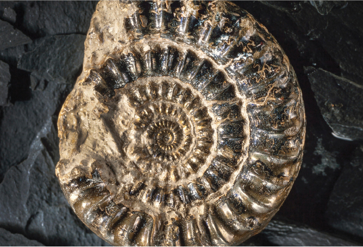
An ammonite fossil. Spiraling inward like a snail shell, the fossil is composed of many small chambers laid side-by-side.
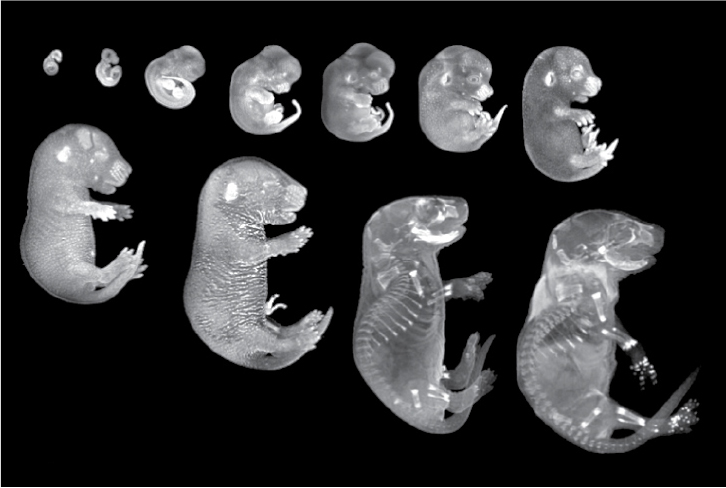
Eleven images of mouse embryos, arranged in order of size. The smallest looks like a bean, while fully formed bone structure and identifiable body parts are evident in the largest.
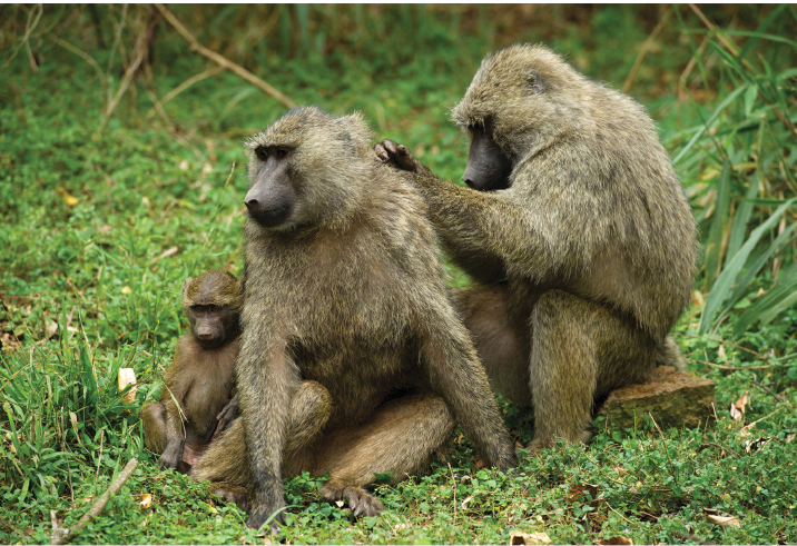
Two adult baboons and one juvenile on a grassy slope. One adult is grooming the other.
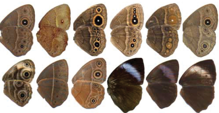
Twelve halves of butterfly wings, laid outside by side in two rows of six each. A variety of eye-like circular spotting patterns is evident, as well as numerous variations in color.
A blue film composed of many parallel lines, with dark bars of spotting at some points. A hand holding a pen appears in silhouette, hovering above the film.
At its core, evolutionary biology is the study of the origin, maintenance, and diversity of life on Earth over approximately the past 3.5 billion years. To understand the evolution of a species fully, we need to know the ancestral species from which it descended, and we need to know what sort of modifications have occurred along the way. Darwin referred to this entire process as descent with modification.
One of the most important processes responsible for the modifications that occur over time is natural selection. We will discuss natural selection and other evolutionary processes in greater detail in later chapters. For now, we can summarize the process of natural selection as follows. Genetic mutations, or changes to the DNA sequence, arise continually and can change the phenotype—the observable, measurable characteristics—of organisms. These mutations can increase fitness, decrease fitness, or have no effect on fitness, where fitness is measured in terms of relative survival rates and reproductive success. Most mutations will disrupt processes that are already fine-tuned, and thus they will have harmful effects on fitness. By analogy, consider tinkering with a computer program. If you randomly change one line of code, chances are that you will break the program entirely, degrade its performance, or, at very best, have no effect on the program’s function. But sometimes you will get lucky—your change may actually improve the program’s operation. Genetic mutations are similar. Most are deleterious or neutral, but by simple luck some mutations turn out to be advantageous in the sense that the individuals who carry them may have more surviving offspring than average. Such genetic changes that improve the fitness of individuals will tend to increase in frequency over time.
The result is evolutionary change by natural selection. Advantageous genetic changes, accumulated over long periods of time, can produce dramatic effects within a population, even to the extent of producing new species, genera, families, and higher taxonomic orders. Indeed, as we will see many times throughout the course of this book, the process of natural selection is fundamental in what are called the major transitions in evolution—the evolution of the prokaryotic cell, the evolution of the eukaryotic cell, the evolution of multicellularity, and so on—that have taken place over the past 3.5 billion years of life on Earth.
Throughout this book, we will examine the power of natural selection in shaping the life that we see around us. We begin with some of the practical applications of understanding evolution via natural selection. Then we examine phylogenetics. The examples in these sections, as well as all the examples we discuss in this chapter, illustrate some of the major concepts, methods, and tools that biologists use to understand evolution.
The next time you sit down for a meal, look at the items on your plate. Whether you’re enjoying a home-cooked supper or fast-food takeout, the food you are eating is almost certainly the product of evolutionary change from intense selective breeding over time. Indeed, humans have been selectively breeding grains, such as barley (Hordeum vulgare) and wheat (Triticum aestivum), as well as lentils (Lens culinaris), foxtail millet (Setaria italica), and peas (Pisum sativum), for more than 11,000 years (Figure 1.2) (Larson et al. 2014; MacHugh et al. 2017; Frantz et al. 2020).
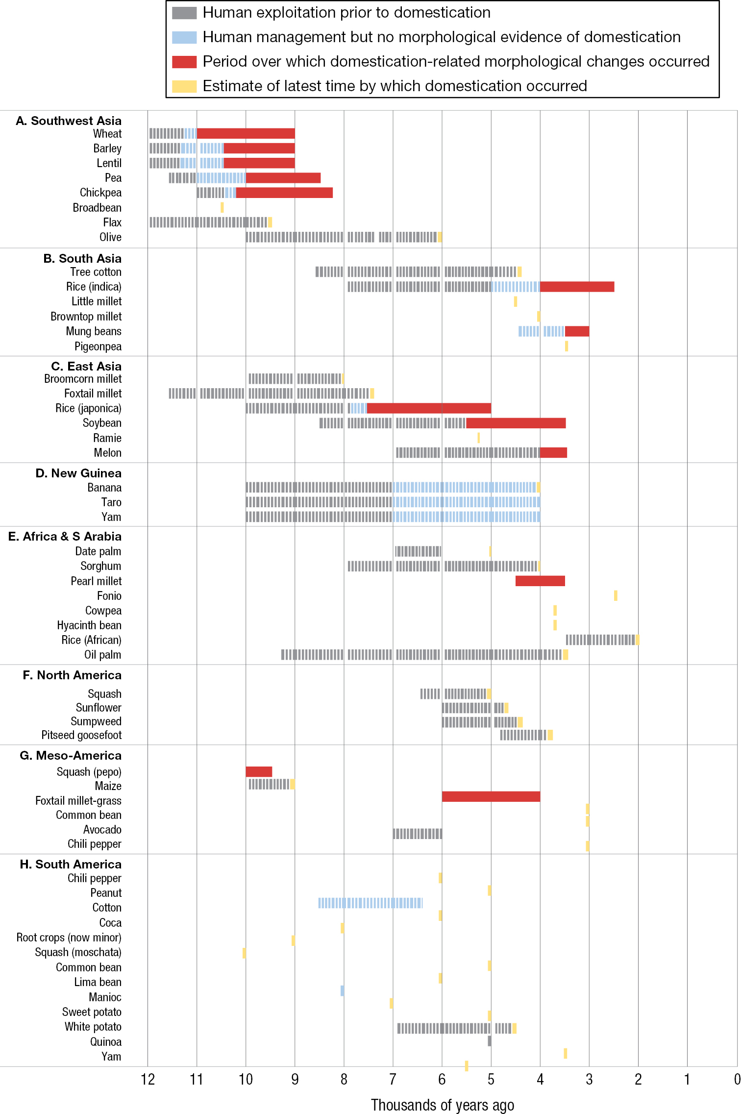
A horizontal bar graph of plant domestication by geographic region. The horizontal axis measures years before the present era, or B P for short, and ranges from 0 to 12000. The vertical axis lists about 50 species. A bar indicates the period of pre-domestication use and period of domestication for each species listed. Southwest Asia features the earliest periods of domestication, ranging from a period from 11000 to 9000 years B P for wheat to a latest possible date of domestication at 6000 years B P for olives. The species domesticated earliest in South Asia is little millet, 4500 years B P, while the most recent is indica rice, from 4000 to 2500 years B P. The species domesticated earliest in East Asia is broomcorn millet, from 8000 years B P, while the most recent is melon, from 4000 to 3400 years B P. The domestication events recorded for New Guinea are those of the banana, the taro, and the yam, all of which entered use 10000 years BP and were done being domesticated by 4000 years B P. The species domesticated earliest in East Africa and South Arabia is the date palm, 5000 years B P, while the most recent is African rice, 2000 years B P. The species domesticated earliest in North America is the squash, with a latest possible date of domestication of 5000 years B P, while the most recent is pitseed goosefoot, with a latest possible date of domestication of 3800 years BP. The species domesticated earliest in Meso-America is the pepo squash, from 10000 to 9500 years B P, while the most recent are foxtail millet-grass, the common bean, and the chili pepper, all with a latest possible date of domestication of 3000 years B P. The species domesticated earliest in South America is moschata squash, with a latest possible date of domestication of 10000 years B P, while the most recent is the yam, 3500 years B P.
The process of human-directed selective breeding, known as artificial selection, is straightforward. In each generation the “best” plants—for example, those that are the hardiest, quickest growing, most productive, and best tasting—are chosen as the parental stock for the next generation. Because offspring tend to resemble their parents, the population of plants increasingly takes on these beneficial characteristics when this process is repeated over time.
To illustrate this key point, Darwin used strawberries as an example of artificial selection (Figure 1.3). He wrote “As soon, however, as gardeners picked out individual [strawberry] plants with slightly larger, earlier, or better fruit, and raised seedlings from them, and again picked out the best seedlings and bred from them, then, there appeared (aided by some crossing with distinct species) those many admirable varieties of the strawberry which have been raised during the last thirty or forty years” (Darwin 1859, pp. 41–42).
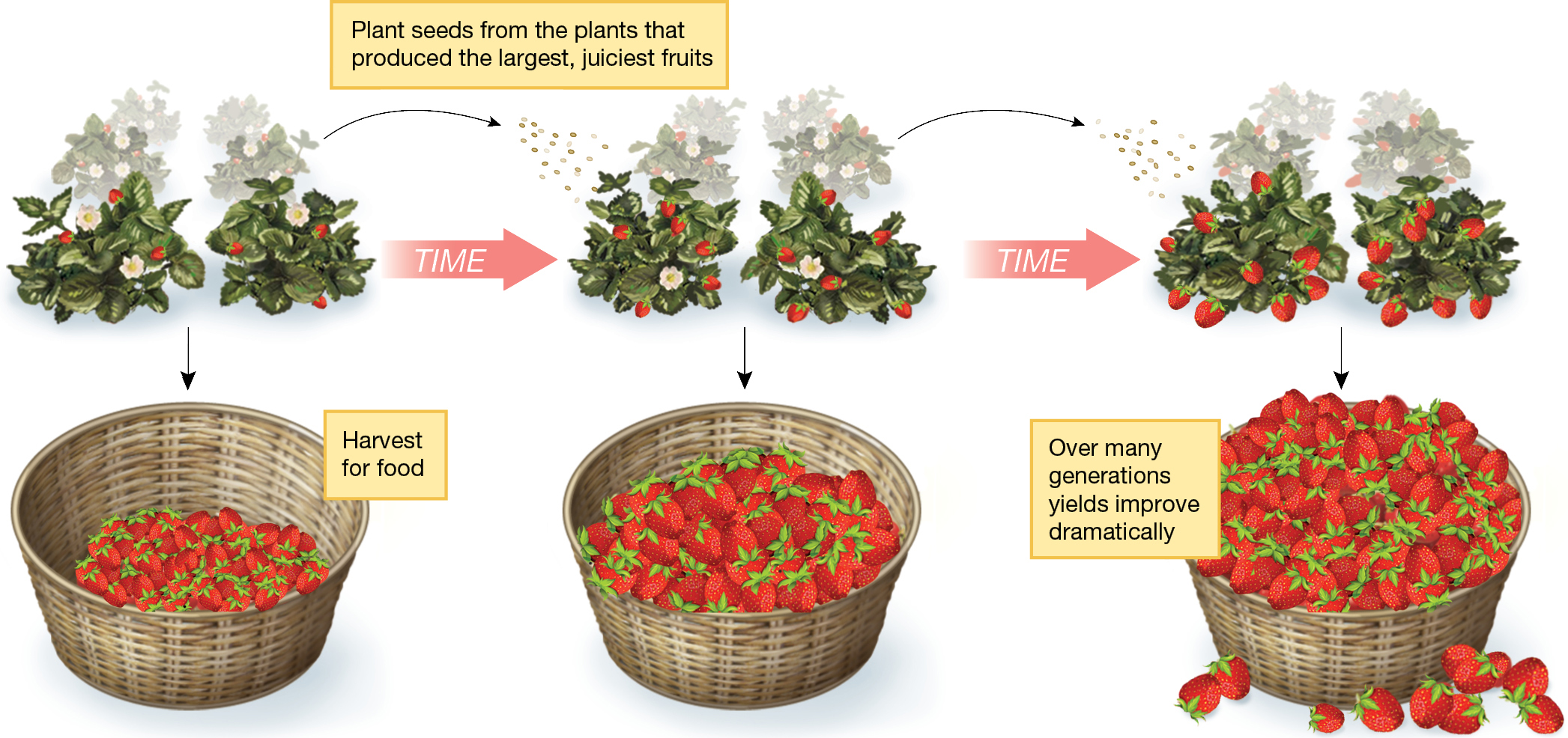
An infographic about strawberry breeding. Three images of strawberry plants are shown, with arrows pointing from each to the next labeled “Time.” Below each set of strawberry plants, an arrow points to a basket filled with picked berries. The yield fills the first basket one third full, the second basket two thirds full, and overflows the third basket. Text reads, “Plant seeds from the plants that produced the largest, juiciest fruits. Harvest for food. Over many generations yields improve dramatically.”
Artificial selection by humans is thus a counterpart to natural selection. With natural selection, traits that are associated with increased survival and reproduction increase in frequency. With artificial selection, humans choose which individuals reproduce, and in so doing, select traits that are in some way beneficial to us. Such selective breeding can produce dramatic results. For example, the productivity of wheat, rice, and corn has doubled since 1930; much of that increase arose from selection of genetic crop strains better adapted to their agricultural environments. And the same holds true when we look at the selective breeding of animals, which has resulted in increased egg production by chickens and increased milk production by dairy cows.
Even as artificial selection improves the quality and yield of crops and livestock, other evolutionary changes have detrimental effects on the human food supply, as we see with pesticide resistance. Although the Food and Agriculture Organization of the United Nations estimates that 20% to 45% of all crops globally are still lost to insect damage each year, and that number may increase as global warming results in increased population sizes in crop pests, the development of pesticides was a major breakthrough in reducing crop pests and thereby increasing crop productivity (Savary et al. 2019; Deutsch et al. 2018). Natural selection, however, will tend to favor crop pests that are most resistant to such pesticides—as has occurred with diamondback moths (Plutella xylostella) evolving resistance to many of the most frequently used insecticides (Vergauwe and De Smet 2020; Zhu et al. 2017; Troczka et al. 2015). The result is an “arms race” between pest species that feed on crops and humans determined to get rid of such species (Furlong et al. 2013; Chattopadhyay et al. 2020). Resistant pests increase in frequency, and humans continue with ever-stronger insecticides. Evolutionary change occurs quickly in insects because of their short generation times, and thus humans often lose this arms race.
Given that humans are the ones producing and distributing the pesticides, you might think the evolution of pesticide resistance would be an example of artificial selection. It’s not. The distinction between artificial and natural selection refers not to whether human activity is involved, but rather to whether humans deliberately choose which individuals will reproduce. In the case of increasing grain yields, humans actively select those varieties with higher yield. In the case of increasing pesticide resistance, humans produce the pesticides but do not deliberately choose pesticide-resistant strains of insects for further reproduction. Indeed, what we want—pests easily killed by our pesticides—is just the opposite of what natural selection produces. Desirable or otherwise, evolutionary change due to human activity is called anthropogenic evolution (Carroll et al. 2014). In a world shaped by climate change, habitat destruction, environmental pollution, overfishing, and other human influences, anthropogenic evolution is ubiquitous. Later in this chapter, and throughout this book, we will look at more of the ways that human activity is driving evolutionary change in natural populations.
One theme that we will return to repeatedly throughout this book is the manner in which research in evolutionary biology can inform our understanding of disease and help us to design more effective responses to the problems associated with disease. For example, the discovery and development of antibiotic drugs for preventing or treating bacterial infections was one of the major medical developments of the twentieth century. But ever since humans first began using antibiotics, medical practitioners have had to deal with bacteria that are resistant to these drugs. The first modern antibiotic, penicillin, was introduced clinically in 1943; within a single year, penicillin resistance was observed, and within 5 years it had become common in several bacterial species. Since then, numerous new antibiotics have been developed and introduced to the market, only to lose their effectiveness within a matter of years as bacteria evolved resistance to the drug (CDC 2019) (Figures 1.4 and 1.5). The spread of antibiotic resistance is the result of anthropogenic evolution.
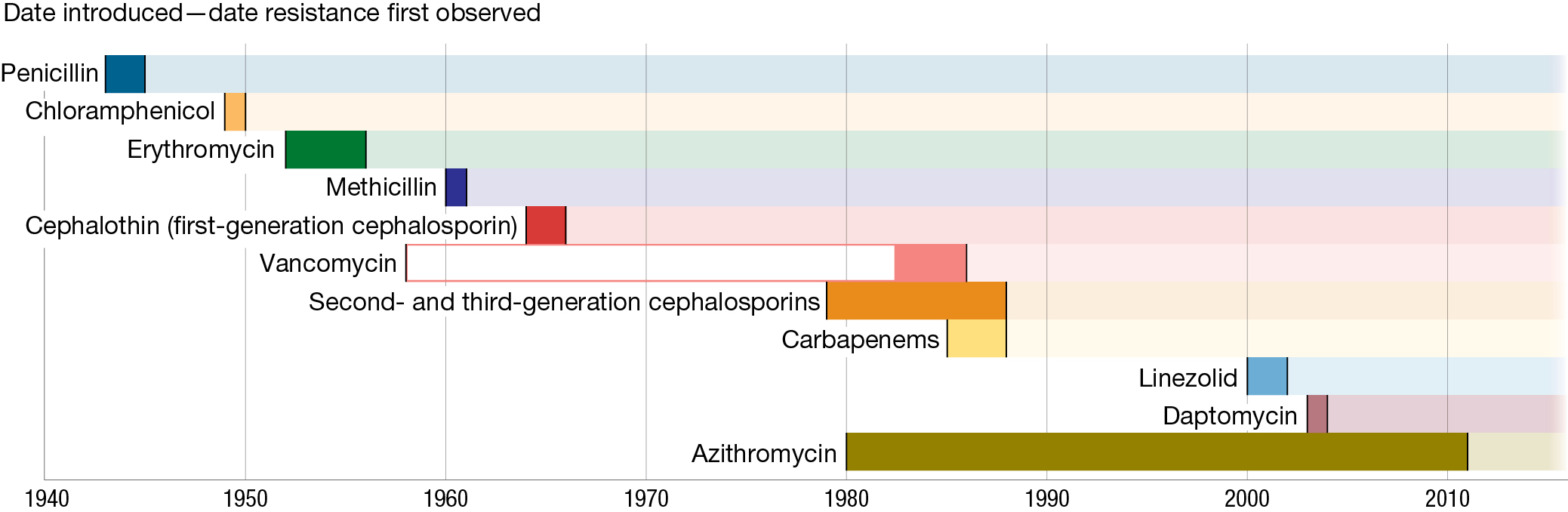
A timeline illustrating antibiotic introduction and resistance. On the timeline, penicillin and chloramphenicol were introduced in the 1940s, erythromycin in the 1950s, methicillin and first-generation cephalosporin in the 1960s, and vancomycin and carbapenems in the 1980s. Linezolid and daptomycin were introduced in the 2000s, and ceftazidime-avibactam in the 2010s. With every one of those types of drugs, resistance was observed within five years. Second- and third-generation cephalosporins were introduced in the 1970s, and resistance was observed in about eight years. Azithromycin was introduced in the early 1980s and, unusually, remained in use for three decades before resistance was first observed.
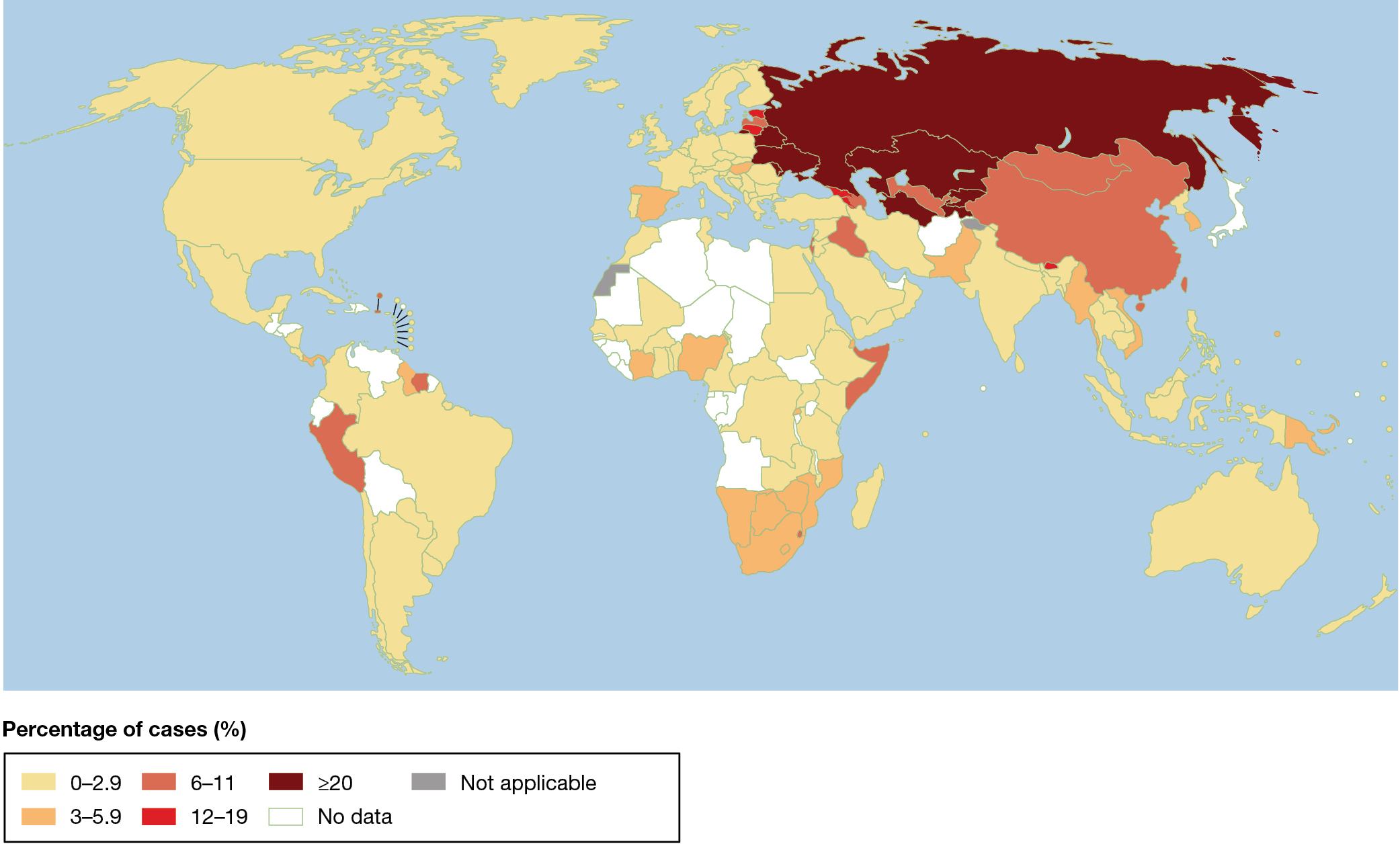
A world map illustrating the geographic distribution of drug-resistant tuberculosis in 2020. The most cases were observed in Russia, Kazakhstan, Ukraine, and several other countries in Eastern Europe and Southwest Asia, where in over 20 percent of all new cases of tuberculosis the mycobacterium was resistant to multiple antibiotics. Between 12 and 19 percent of new cases were resistant in Estonia, Lithuania, Georgia, Armenia, and Bhutan. Between 6 and 11 percent of new cases were resistant in China, Mongolia, Iraq, Israel, Somalia, and Peru, and a few other nations.
Bacteria reproduce at an astounding rate—in some cases, as frequently as once every 20 minutes. They reach enormous population sizes—a single gram of feces can contain 100 billion bacteria—which offer plentiful opportunities for mutations that confer resistance to arise. Antibiotics impose very strong natural selection for resistant strains. For all of these reasons, bacteria can evolve extremely rapidly, and when they are exposed to antibiotics, this is precisely what they do.
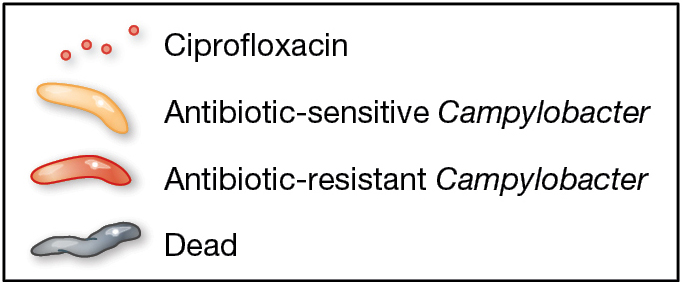
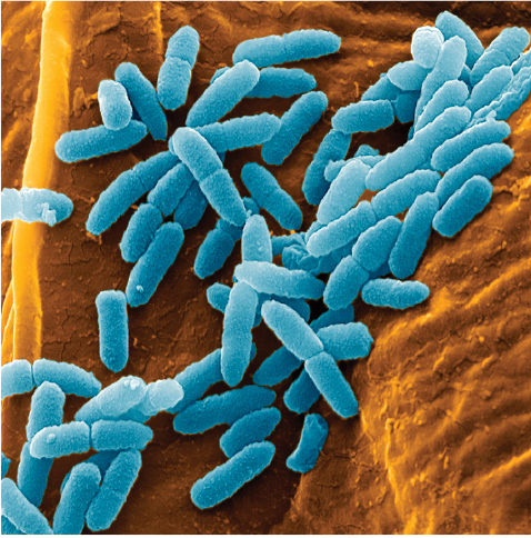
Imagine watching the evolution of resistance to the antibiotic ciprofloxacin. Among other uses, ciprofloxacin is often prescribed for severe cases of food poisoning by the bacterium Campylobacter jejuni. This bacterium is common in the intestines of livestock, where it causes no symptoms, but it can cause acute food poisoning in humans who acquire it by eating contaminated meat. At the start of the process, the gut of a single infected human patient houses millions or even billions of Campylobacter cells that are exposed to ciprofloxacin. Initially, the antibiotic may be deadly to these cells. But with vast numbers of bacterial cells exposed to the antibiotic, and with each cell dividing quickly, it is only a matter of time until a mutation appears that creates a strain of Campylobacter cells that are somewhat resistant to our antibiotic. In a patient being treated with ciprofloxacin, this new strain can outcompete the susceptible strain, and the resistant Campylobacter strain will eventually predominate. Soon another genetic change occurs, producing a strain of Campylobacter that is even more resistant to the antibiotic, and that strain quickly takes over. Repeating this process over and over results in a strain of Campylobacter that is highly resistant to the antibiotic (Figure 1.6).
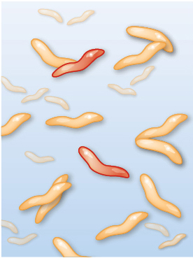
Three illustrations of how Campylobacter interacts with ciprofloxacin. In the first illustration, ciprofloxacin has not yet been introduced to the bacteria culture. Most Campylobacter microbes, which appear as small worm-like cells, are sensitive to antibiotics, only two are resistant, and none are dead. In the second illustration, ciprofloxacin has been introduced. Many Campylobacter microbes are dead, few antibiotic sensitive cells remain alive, and three resistant cells are present. In the third illustration, antibiotic-resistant Campylobacter dominate the population.
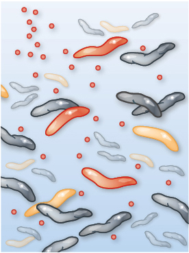
Three illustrations of how Campylobacter interacts with ciprofloxacin. In the first illustration, ciprofloxacin has not yet been introduced to the bacteria culture. Most Campylobacter microbes, which appear as small worm-like cells, are sensitive to antibiotics, only two are resistant, and none are dead. In the second illustration, ciprofloxacin has been introduced. Many Campylobacter microbes are dead, few antibiotic sensitive cells remain alive, and three resistant cells are present. In the third illustration, antibiotic-resistant Campylobacter dominate the population.
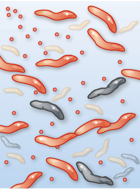
Three illustrations of how Campylobacter interacts with ciprofloxacin. In the first illustration, ciprofloxacin has not yet been introduced to the bacteria culture. Most Campylobacter microbes, which appear as small worm-like cells, are sensitive to antibiotics, only two are resistant, and none are dead. In the second illustration, ciprofloxacin has been introduced. Many Campylobacter microbes are dead, few antibiotic sensitive cells remain alive, and three resistant cells are present. In the third illustration, antibiotic-resistant Campylobacter dominate the population.
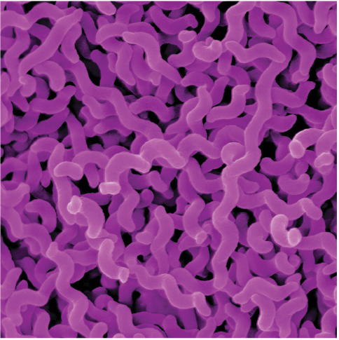
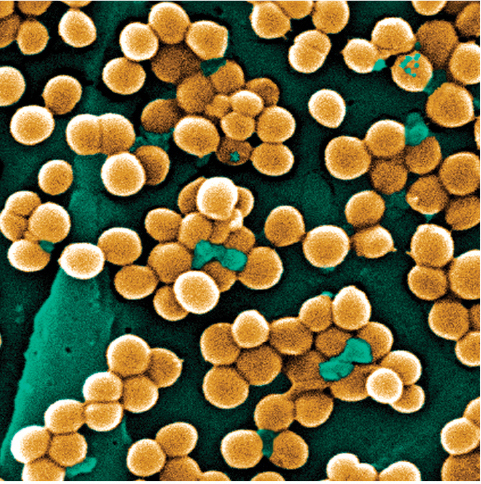
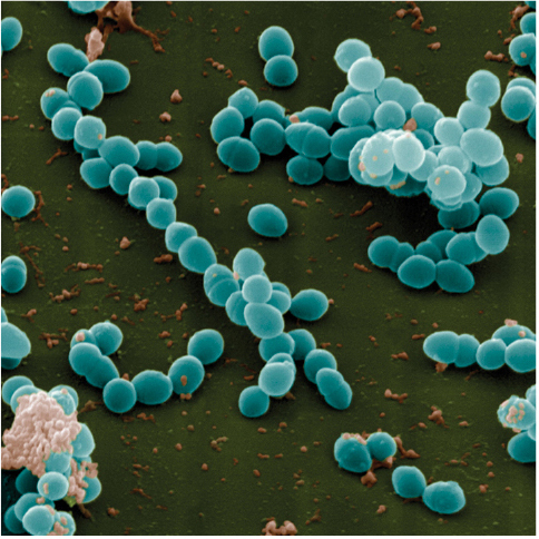
Four photographs of bacteria. The first is Campylobacter jejuni. The cells in the cluster, stained pink, are corkscrew-shaped. The next is Staphylococcus aureus. The cells, stained yellow, are roughly clustered into groups of about 10 cells. Each cell is shaped like a circle. The next is Enterococcus faecalis. The cells are gathered into clusters. Stained blue, they are ball-shaped. The last is Pseudomonas aeruginosa. The cells, stained blue, mainly cluster into pairs.
Although Campylobacter is rarely life threatening, its consequences are certainly dramatic when considered in aggregate: treatment failures resulting from antibiotic resistance are estimated to be responsible annually for nearly 500,000 additional days of diarrhea (Travers and Barza 2002; Quintel et al. 2020). Other antibiotic-resistant bacteria such as Staphylococcus aureus, Enterococcus species, and Pseudomonas aeruginosa pose an even more significant threat (Figure 1.7). In the United States, antibiotic-resistant bacteria cause an estimated 35,000 deaths annually and annual health care costs of nearly $5 billion (CDC 2019; Nelson et al. 2021).
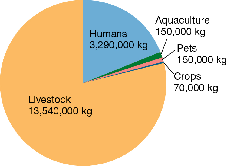
A pie chart illustrating antibiotic use. Over three quarters of all antibiotics are used in livestock, or 13,540,000 kilograms annually. Under one quarter of all antibiotics are used by humans, at 3,290,000 kilograms annually. The remaining uses detailed are in pets, at 150,000 kilograms annually, aquaculture, also at 150,000 kilograms annually, and crops, at 70,000 kilograms annually.
The study of evolutionary biology allows us to understand how antibiotic resistance evolves in these bacteria; this understanding in turn helps us deal with the health threat that such bacteria pose. In the course of drug development, pharmaceutical companies routinely screen potential new antibiotics by exposing bacteria to a wide range of antibiotic concentrations in an effort to find drugs to which antibiotic resistance does not readily evolve. Physicians often prescribe antibiotics in combination because drug combinations decrease the rate at which antibiotic resistance evolves; even if the mutations needed for resistance to one drug should arise, the other drug may kill these bacteria before they can spread. In Europe, the agricultural use of many antibiotics has been banned now that we understand how antibiotic-resistant strains of bacteria can evolve in farm animals and then spread to humans. In January 2022, the European Union enforced even tighter regulations on the use of antibiotics, and more generally on the use of antimicrobial drugs, in agriculture. In the United States, antibiotics are still widely used in agriculture (Figure 1.8). Although the Food and Drug Administration has banned agricultural use of a few antibiotic types, their attempts to curtain agricultural use have largely been ineffectual (Hollis and Ahmed 2013; Hicks 2020).
The use of evolutionary models to address questions relevant to disease is not limited to antibiotic resistance. In subsequent chapters, we will see other examples in which ideas and experiments from evolutionary biology have contributed to a fundamental understanding of the SARS-CoV-2 virus responsible for the COVID pandemic, sexually transmitted diseases such as AIDS, and many other infectious diseases. Evolutionary biology has likewise contributed to our understanding of chronic ailments such as diabetes and obesity and even to an understanding of the phenomenon of aging itself.
Evolutionary biologists hypothesize that all living things have descended from a common ancestor, and over eons the descendants of this common ancestor have diversified to yield the myriad forms that we observe in the world today (Chapter 4). Evolutionary biologists represent the historical relationships among living things with a phylogenetic tree (Figure 1.9). Often, each tip of a phylogenetic tree represents a species that is currently living or a species that has gone extinct, but tips can sometimes represent larger groups—genera, families, orders, and so on—or smaller groups, such as a variant strain of a virus. Branch points on a phylogenetic tree represent points of divergence—events associated with the origin of a new lineage—that occurred in the past. This branching pattern of common ancestry and descent is one of the most important conceptual foundations of biology.
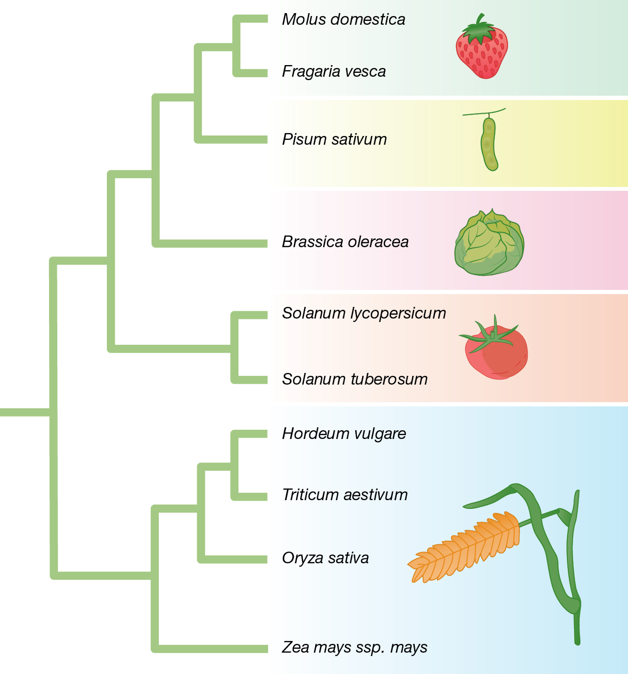
A tree diagram has two main branches. One includes barley and wheat as close relatives, and also rice and corn. The other main branch has a sub-branch that includes tomatoes and potatoes as close relatives, and a sub-branch that includes apples and strawberries as close relatives, and also cabbage and peas.
We can view all species that live or ever have lived as forming a vast branching tree of relationships known as the tree of life (Figure 1.10). The tree of life provides us with a map of the history of life, a map that reflects the evolutionary processes gave rise to all living forms. It connects evolutionary history to the current diversity of life on Earth.
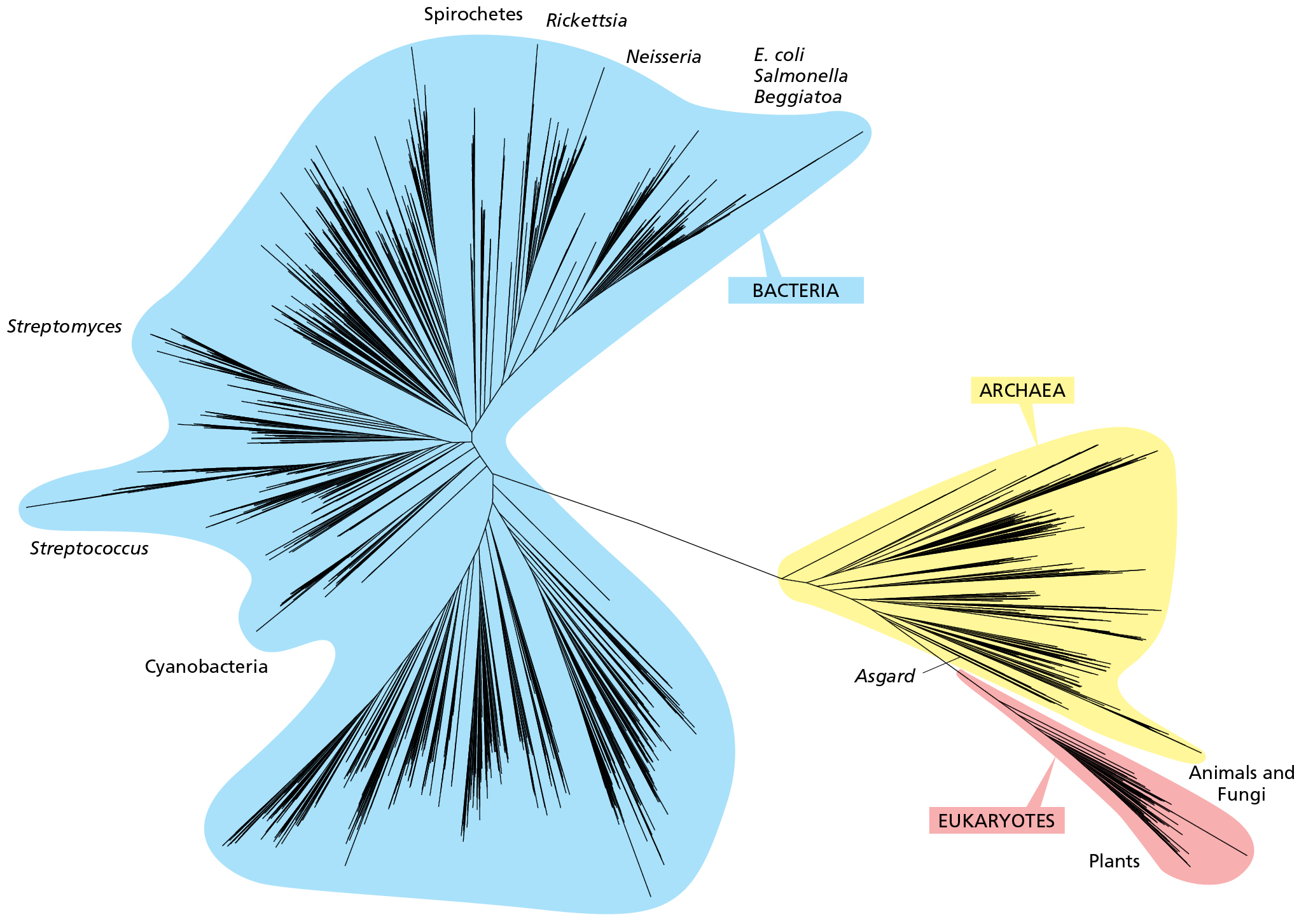
A branching diagram with three main branch clusters. The smallest lobe contains eukaryotes, including animals and fungi, and plants. This lobe branches off from a larger lobe, the archaea, which also contains asgard. The largest lobe contains bacteria, including e coli, salmonella, beggiatoa, nesseria, rickettsia, spirochetes, streptomyces, streptococcus, and cynaobacteria.
An understanding of the tree of life as the product of evolutionary processes tells us about the history of living things, and it also has immediate practical consequences for the world today. For example, phylogenetic thinking provides new ways to conceptualize the challenges of conserving biodiversity. When we think about extinction—that is, the loss of species—we typically focus on the ecological consequences: When a species goes extinct, it disappears from a community or ecosystem where formerly it had occurred. But extinction has evolutionary consequences as well. Each time a species or group of species goes extinct, a part of the tree of life is pruned away, and so part of the evolutionary history of life on Earth is lost (Figure 1.11).
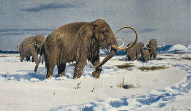
A painting of several woolly mammoths. The shaggy elephant-like beasts have large curving tusks that point back at them and ears that are smaller in proportion than elephant’s ears. They stand in a snowy landscape.
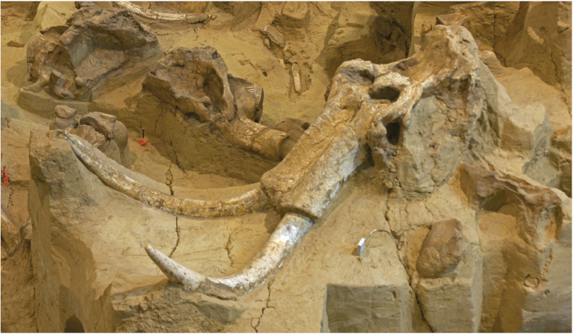
A fossilized mammoth skull on display. The skull and tusks have been uncovered from the surrounding gray substrate. A small square marker has been placed next to the skull.
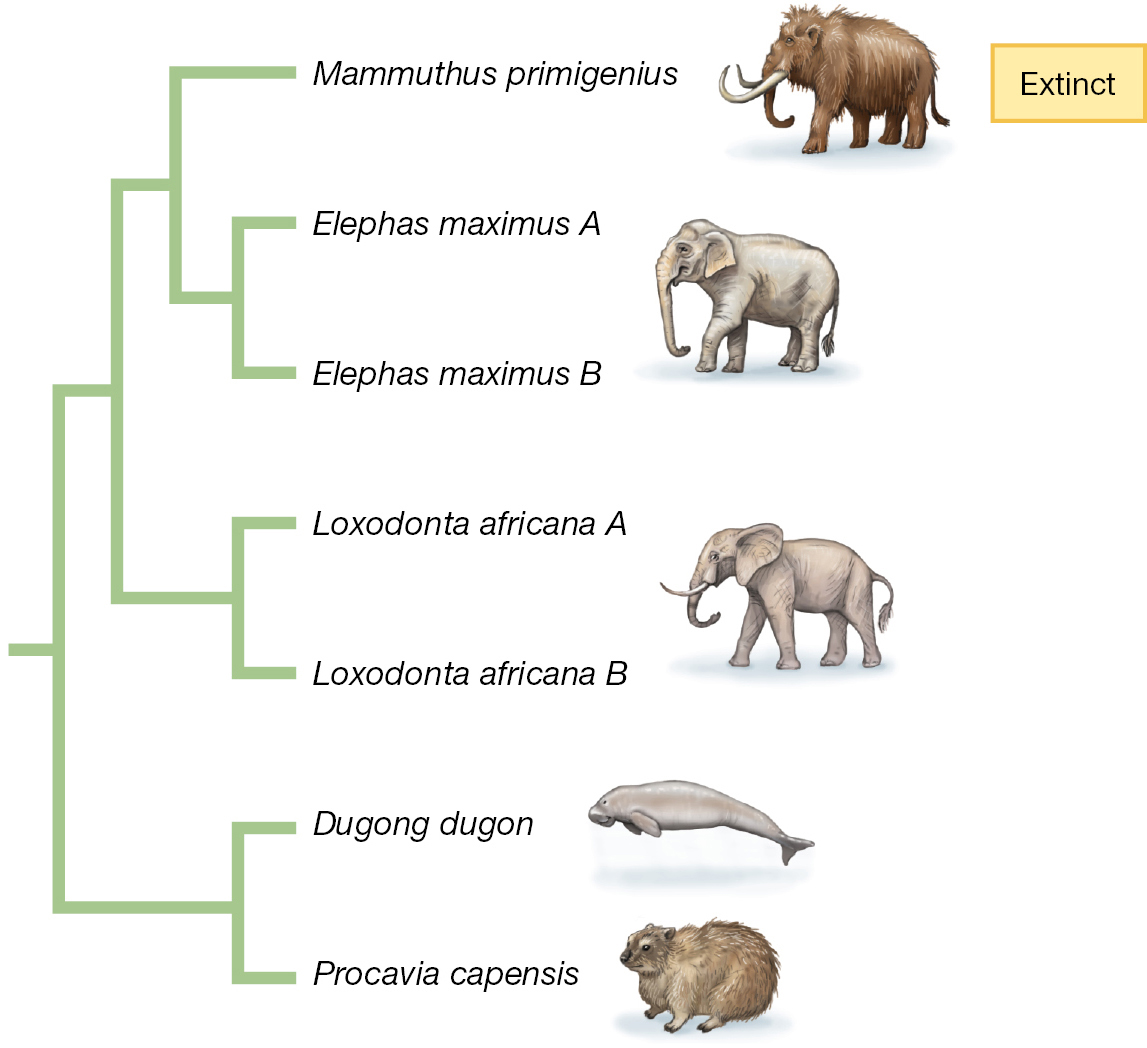
A phylogenetic tree diagram. The right branch of the tree contains a clade containing the species Dugong dugon and Procavia capensis. The left branch of the tree contains a clade containing five species. On the right-hand branch of this clade is the clade containing the species Loxodonta africana A and Loxodonta africana B. The left-hand branch of this clade contains a clade whose left branch is the extinct species Mammuthus primigenius and whose right branch contains the clade containing Elephas maximus A and Elephas maximus B.
As we will emphasize throughout the book, phylogenetic trees are hypotheses and phylogenetic reconstruction is an ongoing process. As new data become available, researchers may reject previous hypotheses and pose new ones. Consider the evolutionary history of a spectacular wading bird called the shoebill (Balaeniceps rex) (Figure 1.12). Superficially, the shoebill looks quite similar to storks, and for this reason, the species is sometimes called the “shoebill stork.” But a phylogeny based on morphological characters published in the 1980s suggests otherwise (Figure 1.13A). This phylogenetic hypothesis places the shoebill as a sister group—a group derived from the same node on a phylogenetic tree—to the herons. In other words, this phylogeny implies the hypothesis that the closest living relative of the shoebill is a heron (Cracraft 1981).
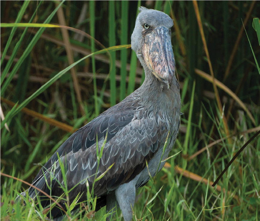
A shoebill stork, with a mottled gray and pink bill like a hugely oversized duck-like bill. The bird’s feathers are gray.
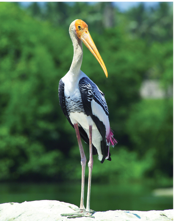
A painted stork, with a long, yellow bill, an orange forehead, a white body, and dark blue and purple patches on its wings.

A great blue heron, with an orange bill and a black stripe on its white head
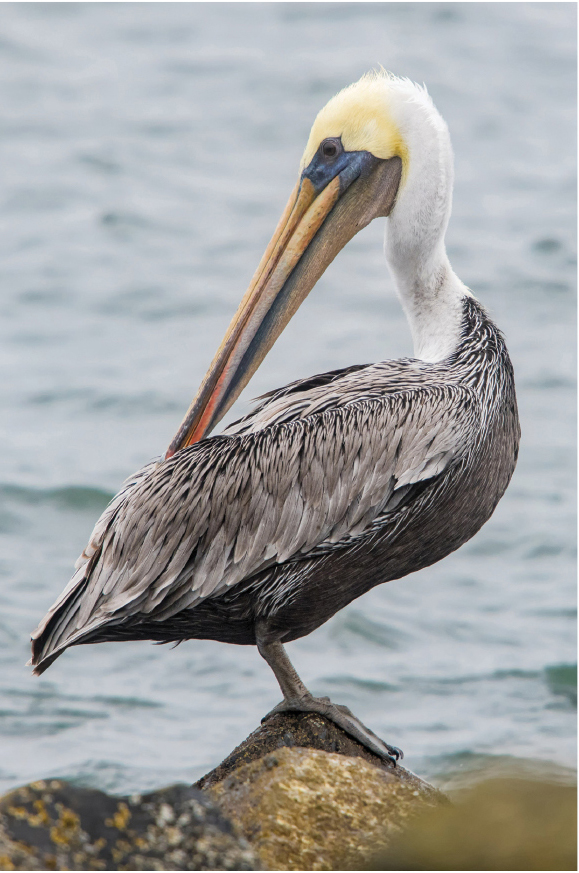
A brown pelican, with a white head and a leathery yellow bill.
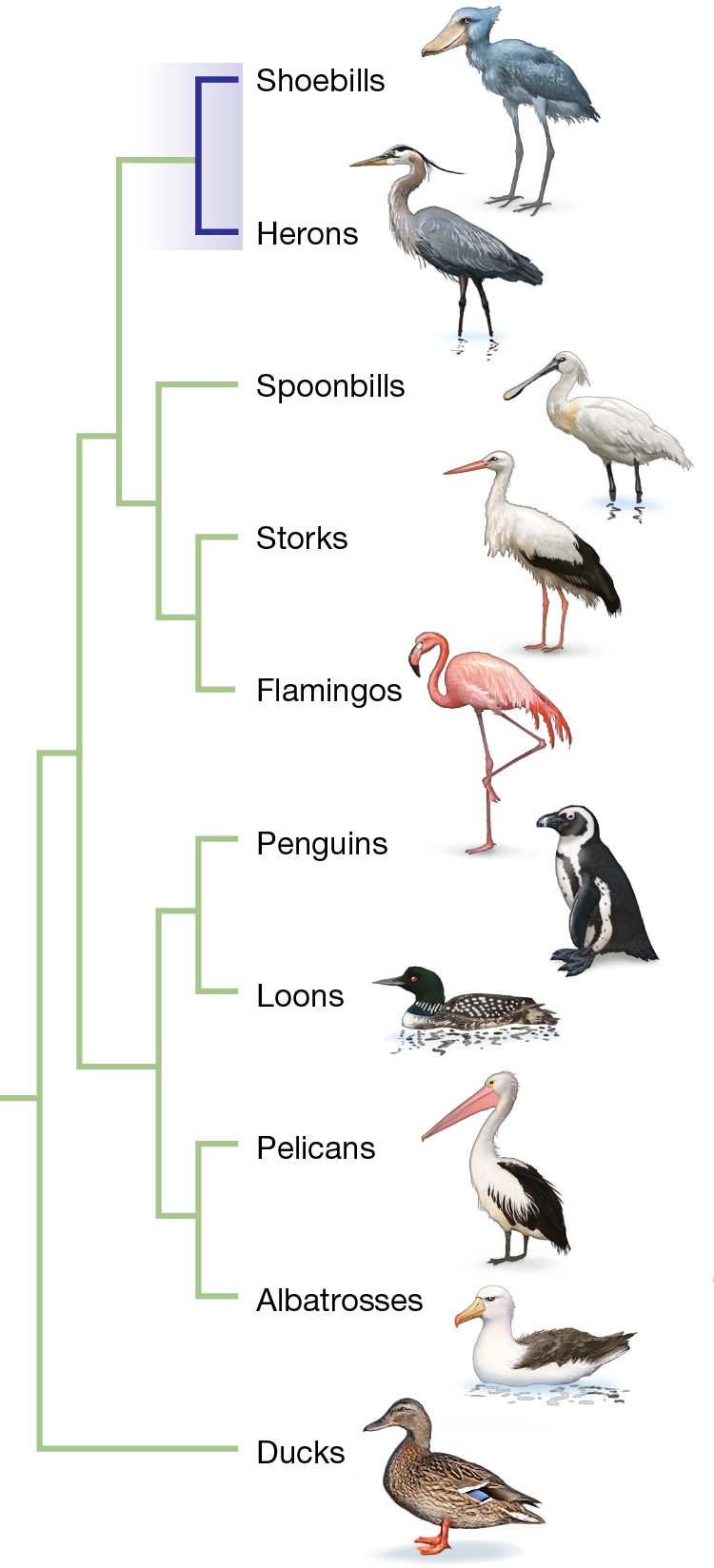
The tree groups shoebills with herons as part of a larger group that also includes spoonbills, storks and flamingos. Other groupings include penguins and loons, and pelicans and albatrosses. Ducks are by themselves.
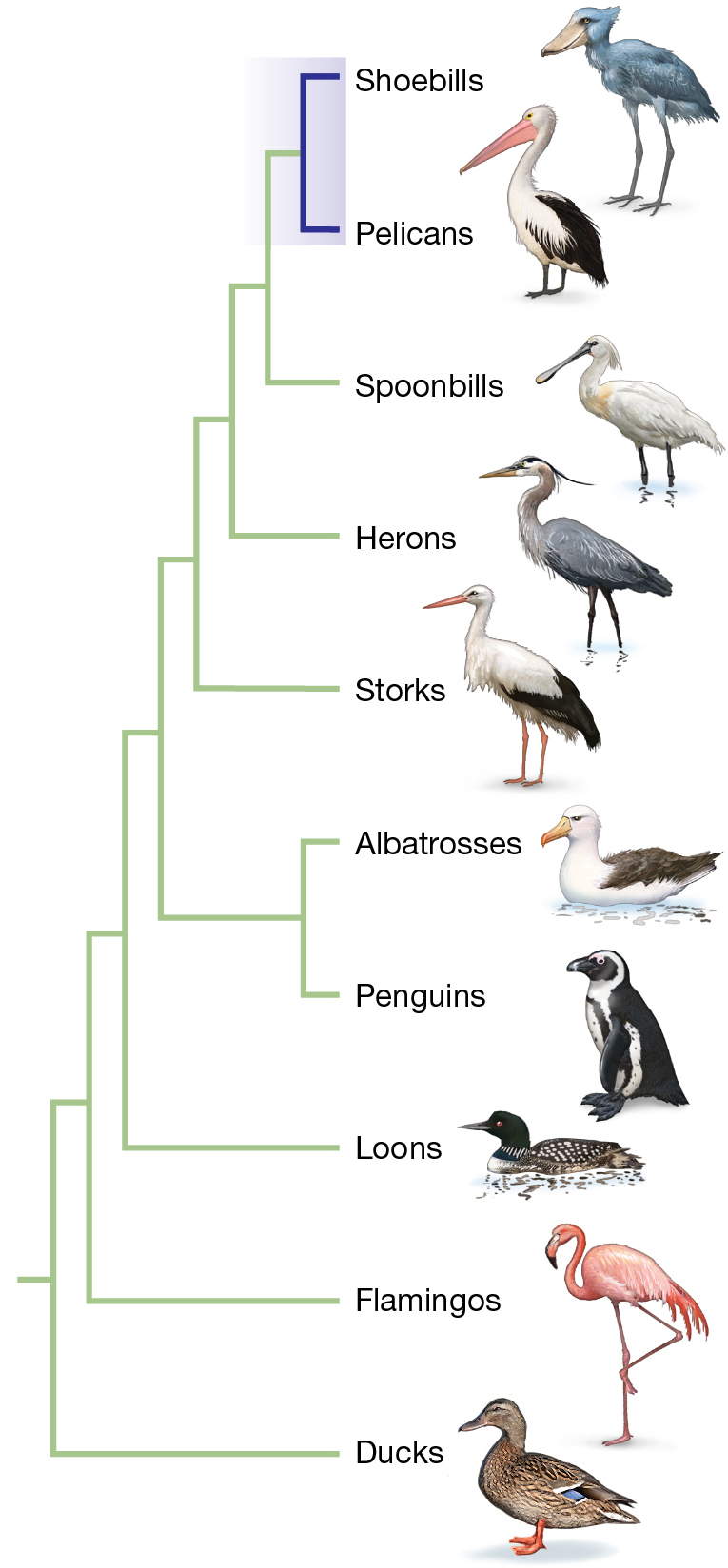
The tree groups shoebills with pelicans and, in order of decreasing relatedness, spoonbills, herons, and storks. More distantly related bird types include albatrosses and penguins, loons, flamingos, and ducks.
As we will explore in greater depth in Chapters 4 and 5, phylogenetic trees can be constructed using many different types of data. Most phylogenetic trees today are based on molecular genetic traits, most often on DNA sequence data. Two decades after the morphological-based phylogeny was published, researchers used molecular genetic data to re-examine the phylogenetic history of shoebills. Figure 1.13B shows a molecular phylogeny of the shoebills (Van Tuinen et al. 2001; Hackett et al. 2008; Jarvis et al. 2014). This tree represents a different hypothesis about the relation among aquatic bird groups. Here, the shoebill is a sister group to the pelicans. In other words, this tree poses the hypothesis that the shoebill’s closest living relatives are pelicans—just as the famous ornithologist John Gould speculated when first describing the species in 1851.
Which tree most likely represents the true phylogenetic history of the shoebill? The evidence is strongly lining up in favor of the hypothesis that pelicans and shoebills are sister groups. Multiple DNA sequencing studies (Van Tuinen et al. 2001; Hackett et al. 2008; Prum et al. 2015; Kuhl et al. 2021) as well as other molecular genetic studies support pelicans as a sister group (Van Tuinen et al. 2001; Kuramato et al. 2015). When more data are gathered—perhaps in the form of whole-genome sequence information—the shoebill’s evolutionary history will be reassessed, as is the case for all phylogenies.
KEYCONCEPT QUESTION
1.1 Even though they are not close evolutionary relatives, why might the shoebill look similar to storks?