“It is too often assumed . . . that profound thoughts can be expressed only in obscure language which the superior minds alone can be expected to understand,” wrote scholar Ronald Englefield (1990). People tend to assume that important ideas must be complex, complicated, and difficult to comprehend. This is not necessarily true. Natural selection, the primary process responsible for generating the remarkable diversity and complexity of all living forms, is conceptually very simple.
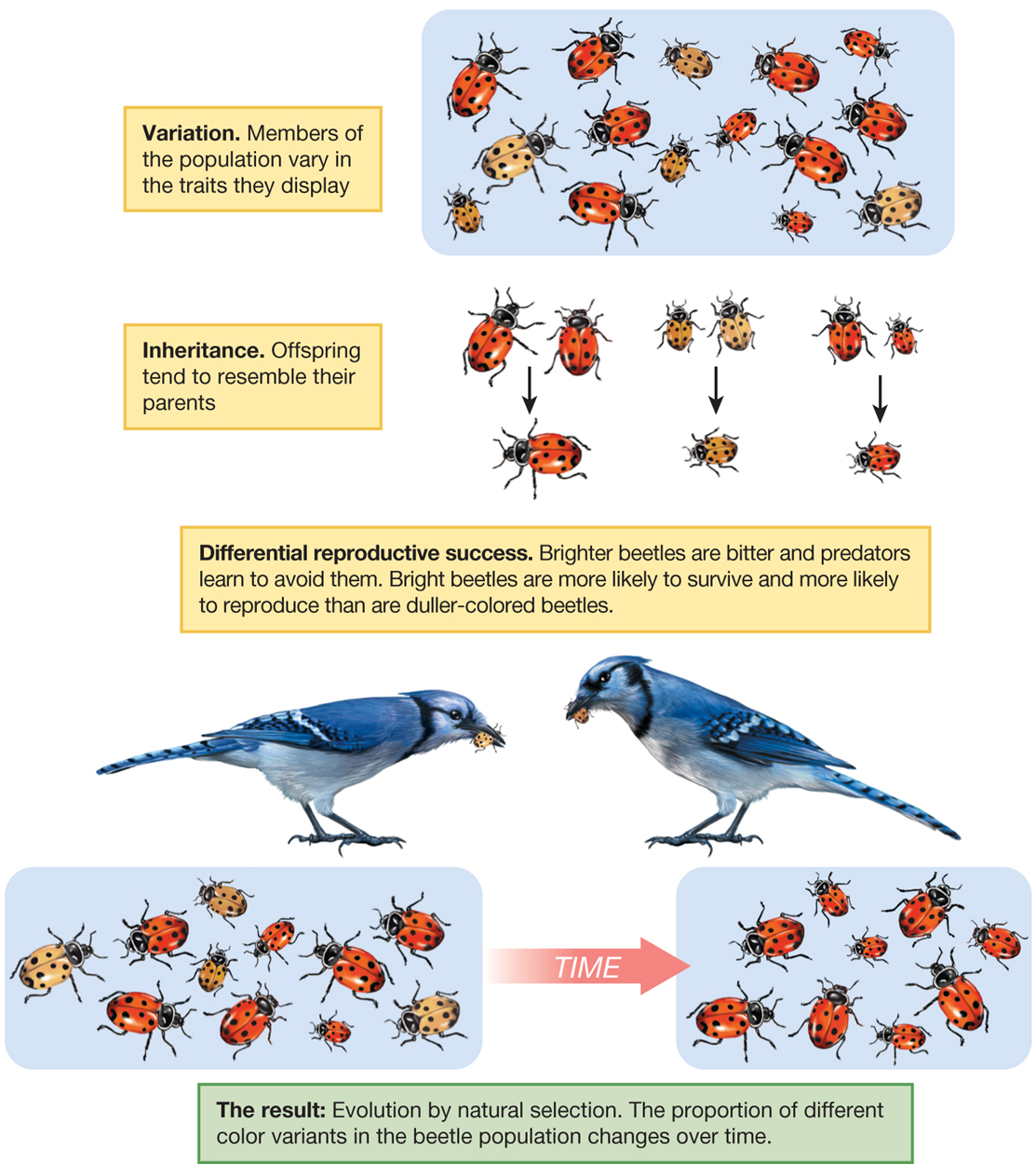
The process of natural selection is inevitable if variation, inheritance, and differential reproductive success are in place (Figure 3.2):
Variation. Individual members of a population differ from one another.
Inheritance. Some of these differences are transmitted from parent to offspring.
Differential reproductive success. Individuals with certain traits are more successful than others at surviving and reproducing in their environment.
More information
A diagram illustrates the three components of natural selection using the example of beetles. The three components are Variation, Inheritance, and Differential reproductive success. Variation means that the Members of the population vary in the traits they display. The diagram includes a group of beetles of all different sizes with different shades of red on their shells. Inheritance is explained as when offspring tend to resemble their parents. There are three groups of beetles from the above group coupled with an arrow pointing down to another beetle. The beetle being pointed to resembles the two beetles above. The third component, differential reproductive success, is exemplified by the fact that brighter beetles are bitter and predators learn to avoid them. Bright beetles are more likely to survive and more likely to reproduce than are duller-colored beetles. Two birds are depicted eating the dull beetles. The result is evolution by natural selection. The proportion of different color variants in the beetle population changes over time. There are now two populations of beetles with an arrow separating them that says time. The first population looks like the population at the top of the diagram with beetles varying with both size and shade of red. After the time arrow, the second population now only varies by size.
FIGURE 3.2The three components of natural selection. Evolution by natural selection occurs when there is variation, inheritance, and differential reproductive success among individuals in a population. Animation: Natural Selection animation
Let’s examine why each is necessary and how together they lead to evolution by natural selection. In so doing, we should keep four points in mind.
Mutations generate variation. Mutation is one of the major sources generating the variation on which natural selection acts. Although some mutations may be favored by natural selection, mutations occur at random with respect to the needs of the organism, independently of whether or not they would be favored by natural selection. We explore this point in greater depth in Chapter 6.
Traits are the object of explanation. When evolutionary biologists study the process of natural selection, they typically focus on how some trait of interest changes or remains constant over time. Researchers can study many different kinds of traits. They often examine a physical characteristic of an organism; for example, the color of a bird’s plumage, the shape of a mammal’s tooth, or the structure of a plant’s flower. Other times, researchers study behavioral traits, such as the elaborate dance of a lyrebird or the predator-avoidance behavior of the sea slug Tritonia. Sometimes the trait will simply be a genetic character: Which sequence of some particular gene does an individual have or how many chromosomes does a species of grass have? Irrespective of the type of trait, most studies of natural selection begin by specifying which trait or traits are to be considered.
Populations, not individuals, change. Natural selection is a process by which the characteristics of a population—not those of an individual—change over time. When we study natural selection, we will typically do so with reference to one or more specified populations of individuals. Thus, in the study of natural selection, traits are usually the object of explanation, and populations are the level of analysis.
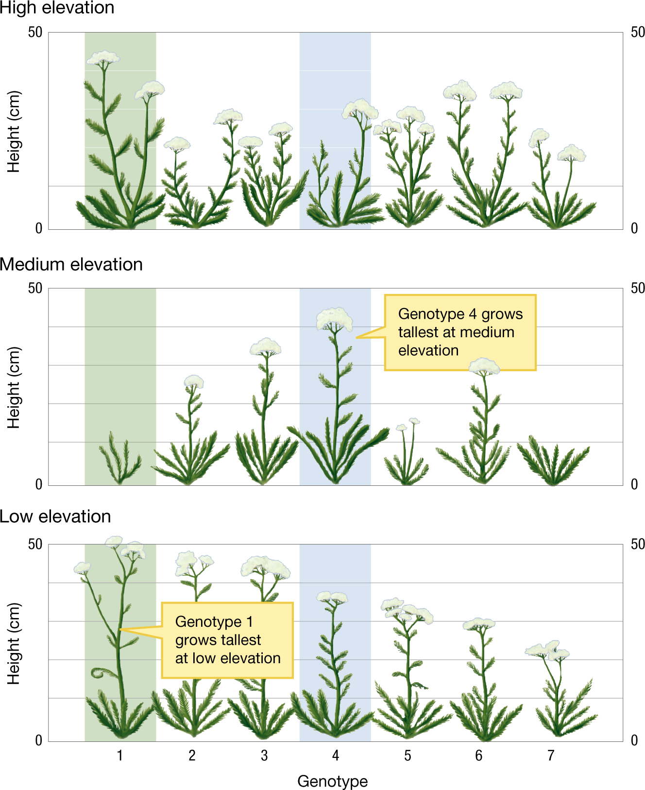
Genotype interacts with environment to produce phenotype. Natural selection does not directly sort on genotypic differences, but rather it sorts on phenotypic differences—the expression of genotypes—among the individuals in a population. Thus, to understand natural selection, we have to understand how the interplay between genotype and environment determines the phenotype. The key here is that a gene by itself does not code for a trait, but rather a gene codes for how a trait is manifest in the context of a particular set of environmental conditions. For example, Figure 3.3 illustrates the way that elevation and genotype interact to determine the height of individuals in different populations of a yarrow plant (Achillea millefolium). In most cases, a genotype does not lead to the production of a single phenotype, but rather produces what we call a norm of reaction. Each column in Figure 3.3 gives us the information we need to construct a norm of reaction for one particular genotype. For example, the column with green shading shows how the heights of plants of genotype 1 depend on the elevations at which they are grown. Genotype 1 doesn’t just produce “tall” or “short” plants. Rather, genotype 1 specifies the norm of reaction “tall at low and high elevations, short at medium elevation.” Norms of reaction are often represented as functions or curves, as illustrated in Figure 3.4. Each genotype is represented by a single curve, showing how expression of a genotype depends on the environmental conditions. Environmental conditions are shown on the x axis, and phenotypes are shown on the y axis. Such norms of reaction can be quite complex, with a given genotype producing different phenotypes across a range of environmental conditions.
A
More information
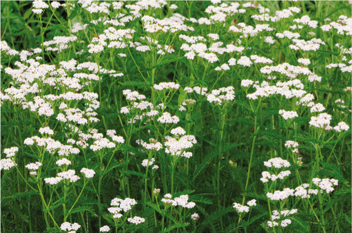
A field is filled with the blooming yarrow plant.
B
More information
Graphs displaying how the height of a yarrow plant depends on both the elevation and its genotype. The graphs are named high elevation, medium elevation, and low elevation with the high elevation at the top and low at the bottom. On the x-axis of all three graphs, the variable, genotype, has a domain from 1 to 7. On the y-axis, height has a range from 0 to 50 in centimeters. The value of the height for each graph is given by the measurement of seven drawings of flowers above each genotype number. The graph for high elevation starts at a maximum of 45 centimeters at genotype 1 then exponentially lowers to 25 centimeters at genotype 3 then exponentially rises again to a local maximum of 37 centimeters, and then drops back off. For medium elevation, the graph is almost symmetric with genotypes at minimums at 10 centimeters and maximized at genotype 4 at 44 centimeters. However, genotype 5 is stunted at 15 centimeters. The low elevation graph starts at the maximum of 52 centimeters and nearly linearly drops to 25 centimeters. There are boxes on the graph pointing out that genotype 1 at low elevation is larger than any of the other genotypes and that genotype 4 on medium elevation is the same way.
FIGURE 3.3Phenotype depends on the effects of both genotype and environment.(A) The yarrow plant (Achillea millefolium). (B) The height of a yarrow plant depends on its genotype and the altitude at which it is raised, as shown by populations of yarrow plants grown in gardens at three sites that were at different altitudes: high, medium, and low elevation. For example, the plants of genotype 1 (green background) grow tall at high and low elevations but are short at medium elevation. The plants of genotype 4 (blue background) have the opposite response to elevation. This genotype grows tallest at medium elevation and shorter at high and low elevations. Adapted from Clausen et al. (1940, 1948).
A
More information
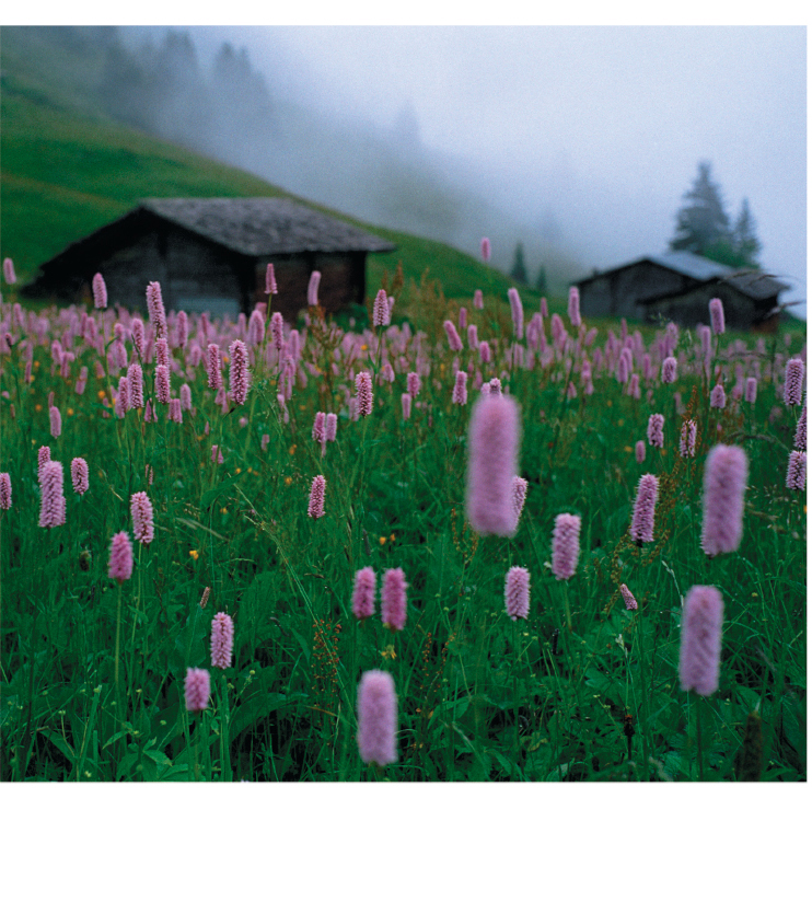
A field of the weedy plant Persicaria maculosa on a foggy day. The plants cover a hill and there are two huts in the background.
B
More information
A line graph of light intensity versus number of leaves. Light intensity goes from 8 to 100 percent. Number of leaves ranges from 0 to 200. There are many lines representing the norm of each specific genotype. Each line is made up of two straight lines that meet at a cusp. This cusp is at 37% light intensity. All the genotypes have about the same number of leaves at 8 percent light intensity (around 25 leaves). Then the lines all increase but also begin to be further and further apart until their cusps are at 37% light intensity. At the cusp, the numbers of leaves range from 100 to 150 leaves. After the cusp, the lines level out and all but one continues to increase. The one that was at 150 leaves actually decreases after its cusp. At 100% light intensity, the number of leaves range from 120 to 175.
C
More information
A line graph measuring Light intensity versus Mean leaf area in square centimeters. The area ranges from 2 to 14 square centimeters. Most of the lines in this one are grouped except for one outlier. The outlier is a red line. All lines are once again made up of two lines meeting at a cusp at 37 percent light intensity. At 8% light, the mean leaf area ranges from 4 to 9.5 square centimeters. The red line is 11 square centimeters. At the cusps, the area ranges from 8.5 to 10 square centimeters with the outlier at 13. Then starting at the cusp, all the lines take a linear decline until 100%. At 100% intensity, the lines all are grouped into a range of 6 to 7 square centimeters. The outlier is at 9 square centimeters.
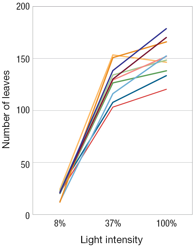
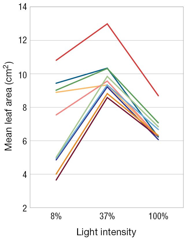
FIGURE 3.4Norm of reaction curves. In the weedy annual plant Persicaria maculosa(A), the total number of leaves (B) and the mean leaf area (C) depend on the light intensity—ranging from full shade to full direct sunlight—that the plant experiences. Each curve for one specific genotype is called a norm of reaction. Here we see the norms of reaction for 10 different genotypes (each a different color), under light intensities of 8%, 37%, and 100% of available sunlight. Thus, the genotypes do not code for a fixed number of leaves or a fixed average leaf size, but rather for a number and size of leaves that depend on the intensity of light to which the plant is exposed. Panels B and C adapted from Sultan and Bazzaz (1993).
Natural Selection and Coat Color in the Oldfield Mouse
With these points in mind, let’s now work through an example of how evolutionary biologists study the process of natural selection. We will focus on an elegant set of studies by Hopi Hoekstra and her colleagues that examines natural selection on coat color in populations of the oldfield mouse, Peromyscus polionotus. This species of small mouse, native to the American Southeast, suffers considerable mortality from predators that hunt visually, such as owls.
Throughout most of its range, P. polionotus individuals are uniformly dark in coloration. But on Santa Rosa Island off the Gulf coast of northern Florida, and along the nearby beaches and barrier islands, these mice often have a much lighter coat color. In this subsection, we will evaluate a number of experiments designed to test the hypothesis that natural selection favors a match between coat color and environmental background, favoring light coat color in the coastal dune populations of P. polionotus that live on light sand and dark coat color in inland populations that live in more vegetated environments (Figure 3.5).
A
More information
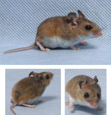
3 photographs of a dark brown mouse with a white belly. Each is from a different angle: front, back, and side.
B
More information
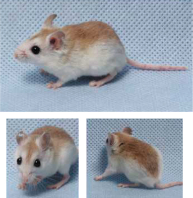
3 photographs of a light brown mouse with a white belly and sides. Each is from a different angle: front, back, and side.
C
More information
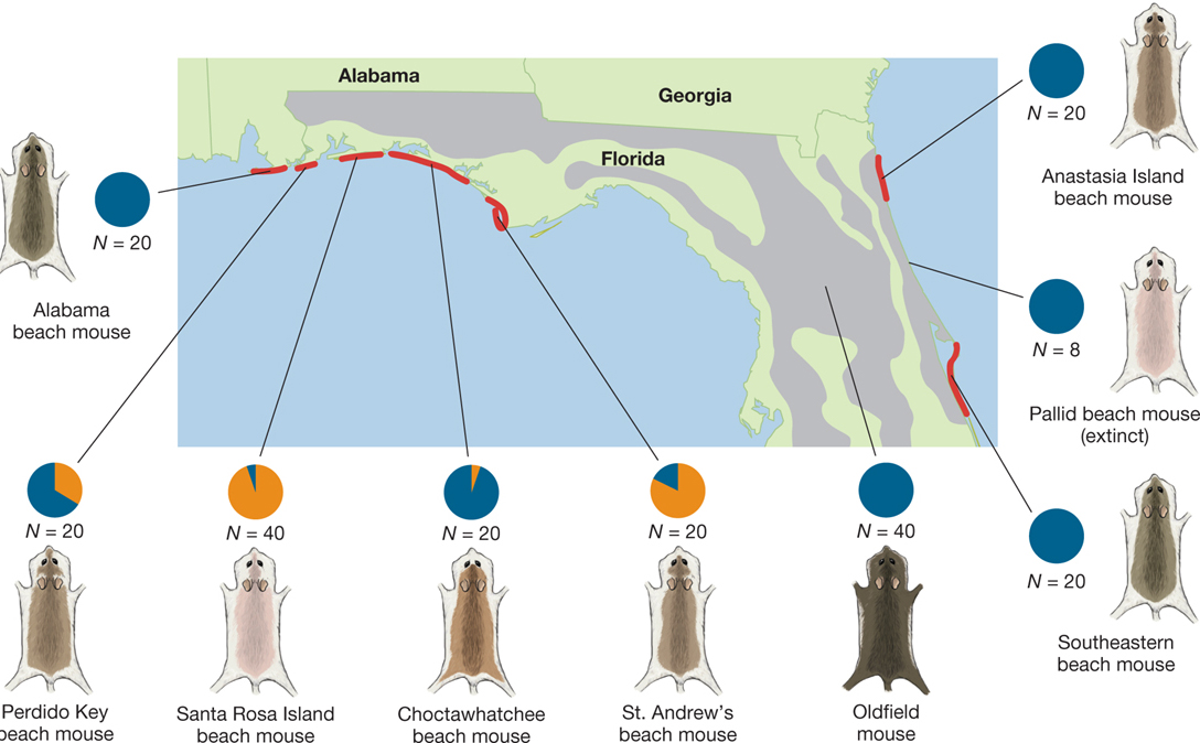
A map of northern Florida and neighboring parts of Alabama and Georgia. It shows where Peromyscus polionotus lives with red spots along the coast and gray areas inland, how the color of its coat changes from place to place, and, with a pie chart, how much of the mouse population had that color of coat. Around the map are pictures of the mice with pie charts showing percent of population. The Alabama beach mouse lives on the Alabama coast just before the Florida line. It has a medium-dark brown coat, and it�s the only color variation of the population. N equals 20. On the Florida coast just after the Alabama line, the Perdido key beach mouse lives. It has a medium brown coat, and its coat color makes up for about two thirds of the mouse population. N equals 20. On Santa Rosa Island, Santa Rosa Island beach mouse lives. It is almost white in color, and it makes up about 10 percent of the mouse population. N equals 40. There is a large section of the map with the red line covering it showing where the Choctawhatchee beach mouse lives, directly east of Santa Rosa Island. It is slightly darker than the Perdido mouse and it makes up 90 percent of the population in that area. N equals 20. Southeast of Panama City is where the St. Andrews beach mouse resides. It makes up about one sixth of the mouse population and is medium brown like the Perdido. N equals 20. In central Florida, near Gainesville, the Oldfield mouse lives and makes up the entire population. It is so dark brown that it almost looks black. N equals 40. On the Atlantic coast east of Orlando, the southeastern Beach mouse lives and makes up the entire population. N equals 20. North of that, and almost exactly east from Greenville is where the Pallid beach mouse used to live but is has now gone extinct. It made up the entire population of mice and it was so light that it almost looked white. N equals 8. The final is the Anastasia Island beach mouse. It lives on the Atlantic coast just south of the Georgia border. It has a medium brown coat and makes up the entire population. N equals 20.
FIGURE 3.5Coat color variation in mice. There are two major color variants of Peromyscus polionotus: (A) the darker inland form, and (B) the lighter beach-dwelling form. (C) Variation in coat color and genotypes at the Mc1R locus. However, P. polionotus exhibits extensive coat color variation across localities in Florida. Red areas indicate the distribution of beach populations; gray areas denote the distribution of inland populations. Characteristic phenotypes for each population are indicated by the coat coloration sketches, but coat color varies within populations as well. The pie charts indicate that the Perdido Key, Santa Rosa Island, Choctawhatchee, and St. Andrew’s beach mouse populations had more than a single variant of the Mc1R locus associated with coat coloration. All populations shown here are considered part of a single species—Peromyscus polionotus. Adapted from Hoekstra et al. (2006) by permission of AAAS.
Now that we have specified our trait of interest—coat color—and our populations of interest—coastal dune and inland populations—we can study the process of natural selection by examining variation, heritability, and fitness in the oldfield mouse.
Variation
Natural selection requires as raw material some variation in the trait under investigation. Without variation, there is nothing for natural selection to select. If, for example, all mice had identically colored coats, natural selection with respect to coat color could not occur.
For a readily observable trait such as coat color, we can easily determine whether the first condition for natural selection—the presence of variation—is satisfied. Hoekstra and her colleagues observed considerable phenotypic variation in coat color within populations (Mullen et al. 2009) (Figure 3.6), and they also uncovered substantial genetic variation at the Mc1R (melanocortin-1 receptor) locus associated with coat color.
More information
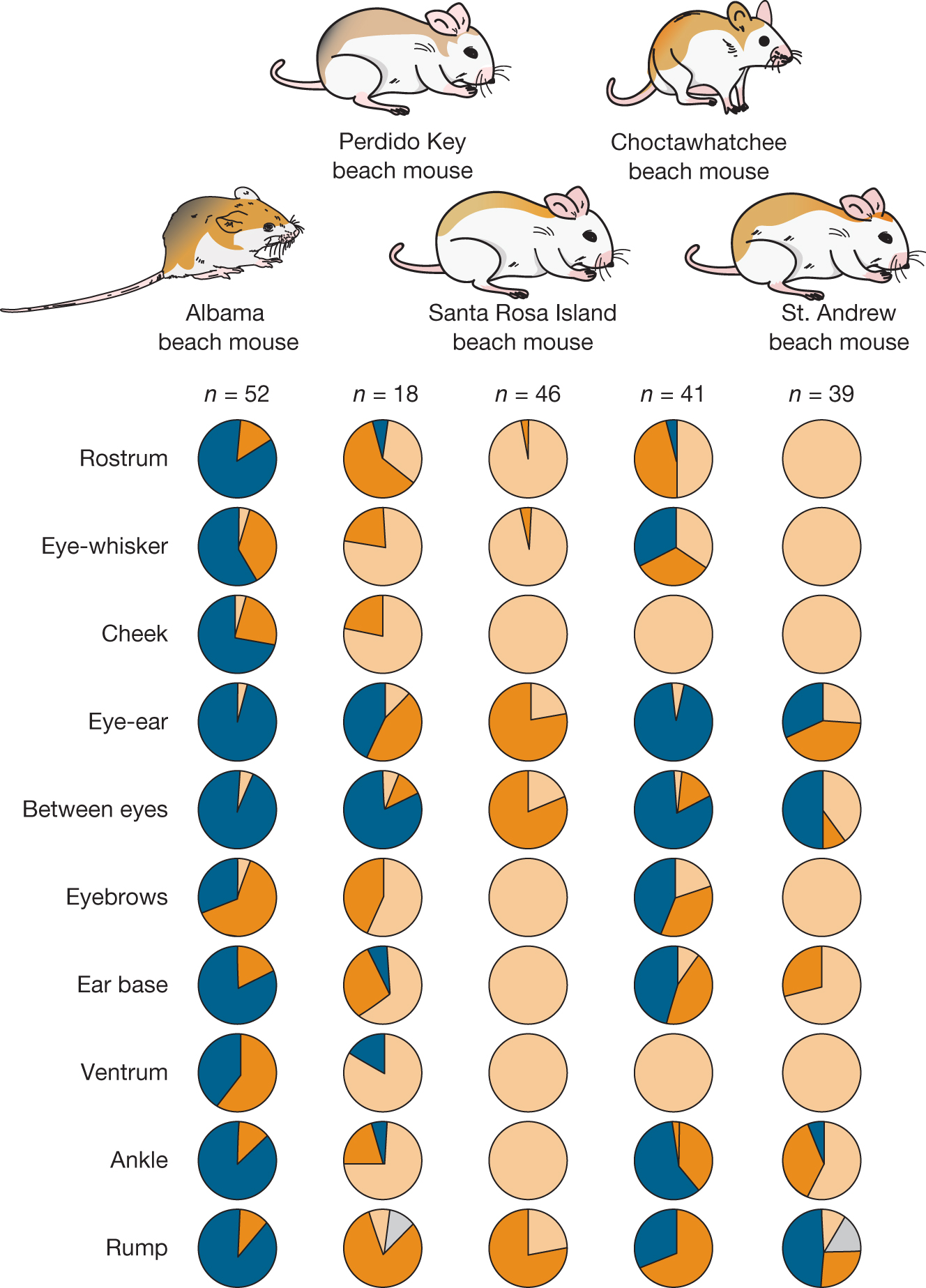
Within-population variation for five separate geographic populations of Peromyscus polionotus, with examination of pigmentation in ten body locations: rostrum, eye-whisker, cheek, eye to ear, between the eyes, eyebrows, ear base, ventrum, ankle, and rump. Alabama beach mouse, N equals 52, is mostly very dark, but over half of individuals have only moderately dark pigmentation in the eyebrows and on the ventrum. Perdido key beach mouse, N equals 18, typically has very dark pigmentation between the eyes and very light pigmentation on the cheek, in the eye-whisker, and on the ventrum. In other locations, pigmentation is more variable. Santa Rosa Island beach mouse, N equals 46, is mostly very light, but over half of individuals have moderately dark pigmentation around and between the eyes, and on the rump. Choctawhatchee beach mouse, N equals 41, typically has very dark pigmentation around and between the eyes and very light pigmentation on the cheek and ventrum. In other locations, pigmentation is more variable. Santa Rosa Island beach mouse, N equals 39, is mostly very light, but about half of individuals have very dark pigmentation between the eyes and on the rump.
FIGURE 3.6Within-population variation in Peromyscus polionotus coloration. Variation in pigmentation traits among five populations of Peromyscus polionotus living on beaches in northwestern Florida. Shading in pie charts represents proportion of individuals with different pigmentation (darker shading = darker pigmentation).
Heredity
Phenotypes result from the interplay of genes and environment. Thus, variation in phenotype can arise through variation in genes alone, variation in environment alone, or through a combination of both. In the case of oldfield mice, variation in coat color could result from genetic differences, from environmental differences such as differences in diets or in exposure to sunlight, or from some combination of these factors. But because offspring inherit genes rather than phenotypes from their parents, natural selection can operate only if there is a genetic component to variation.
Without genetic inheritance, any fitness differences among the varieties of a trait would not result in different frequencies of the trait varieties in the next generation. Imagine that dark-colored mice produce 3 offspring on average and light-colored mice produce 6 offspring on average. If the offspring didn’t resemble their parents with respect to coat color, the dark parents would be no more likely to produce dark offspring than would the light parents, and vice versa. Any consequences of differing reproductive success between coat colors would be lost once the parents produce new offspring.
Most traits that vary do so, at least in part, because of underlying genetic variation. Consequently, almost all traits in natural populations meet the prerequisite for inheritance (Darwin 1868; Endler 1986; Clark and Ehlinger 1987; Mousseau et al. 1999). Indeed, numerous studies from evolutionary biology, population genetics, and animal behavior suggest that many of the traits that in principle could be acted on by natural selection—for example, morphological or behavioral traits—are at least partially inherited from parents by their offspring (Mousseau and Roff 1987; Price and Schulter 1991; Weigensberg and Roff 1996; Hoffmann 1999).
How can evolutionary biologists show that variation in a trait is inherited? The most direct way is to identify the gene or genes responsible for this variation. In the case of the oldfield mouse, Hoekstra and her colleagues have identified several genes that are responsible for much of the coat color variation in P. polionotus (Hoekstra et al. 2006; Steiner et al. 2007). We will consider two of these genes here.
The first of these genes is the melanocortin-1 receptor gene (Mc1R), which produces a protein known to influence coat color in many species of mammals, as well as play a role in plumage color in many species of birds. Mc1R functions as a critical part of a genetic switch that controls the type of pigment that is created and incorporated into hair or feathers (Kronforst et al. 2012). Depending on the environment and the interaction with other genes, this one gene switches back and forth between producing a dark pigment, known as eumelanin, or a light yellow pigment, known as phaeomelanin (Barsh 1996).
Hoekstra and her colleagues have documented a mutation in the Mc1R gene in many of the beach populations of P. polionotus that dwell along the Gulf coast of Florida, where oldfield mice have light coat color (Hoekstra et al. 2006). The mutation reduces eumelanin production, resulting in a lighter coat color. Phylogenetic analysis suggests that this mutation occurred before islands were colonized by beach mouse populations (Domingues et al. 2012).
A second gene involved in coat color in many species is called Agouti. In many populations of snowshoe hare (Lepus americanus), individuals have white coats in the winter, but brown coat color during the rest of the year. In some populations with low snow cover, however, hares remain brown all year. At the genetic level this difference in coat color is the result of differential expression of the Agouti gene (Jones et al. 2018). In oldfield mice, Hoekstra and her colleagues found that beach mice typically carry a recently evolved form of the Agouti allele that contributes to their lighter coat color (Hoekstra et al. 2006). They have also used a technique known as “next generation sequencing” to identify the specific regions of the Agouti gene responsible for light coloration on different parts of the body in oldfield mice and in deer mice (Peromyscus maniculatus) that inhabit the Sand Hills of Nebraska (Manceau et al. 2011; Linnen et al. 2013; Barrett et al. 2019).
Genetic variation alone, however, is not sufficient to allow the process of natural selection to operate. The genetic variation must also correlate with differential reproductive success: genetic variation must have fitness consequences.
Fitness Consequences
While the term fitness has the everyday implication of something that is well matched—or fit—to its circumstances of life, the formal definition in evolutionary biology pertains to reproductive success. The fitness of a trait or allele is defined as the expected reproductive success of an individual who has that trait or allele relative to other members of the population. So, when we speak of fitness here, we are referring to the differential effect of a trait on the expected reproductive success of an individual relative to other individuals in its population (Clutton-Brock 1988; Reeve and Sherman 1993). In many instances, it will be apparent that a trait has an effect on fitness; for the oldfield mouse P. polionotus, we will see below that coat color influences survival. The reason is straightforward. Coat color influences the visibility of mice against their background. Mice that stand out against their background are more readily captured by predators; less visible mice are more likely to survive and reproduce.
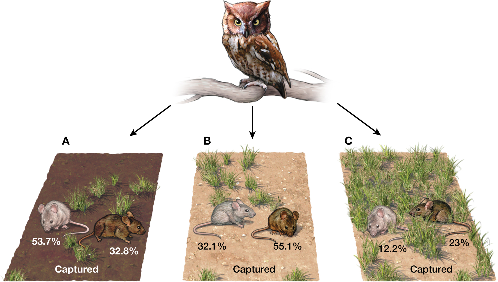
To see the fitness effect of coat color of oldfield mice, let us first examine a 1974 experiment by G. C. Kaufman in which pairs of mice, one with a dark coat and one with a light coat, were released into a large cage with an owl present (Kaufman 1974). For each environmental background—dark soil with sparse vegetation, light soil with sparse vegetation, and light soil with dense vegetation—Kaufman recorded the coat color of the mouse that the owl captured first. Figure 3.7 shows a selective advantage to mice with coats that match the color of their background environment. Those mice were more likely to escape predators and thus to survive long enough to reproduce.
More information
A diagram showing the capture rate of mice from an owl in different colored environments. A. In a dark background with sparse vegetation, light colored mice had a 53.7 percent capture rate, and dark mice had a 32.8 percent capture rate. B. In a light background with sparse vegetation, light mice had a 32.1 percent capture rate and dark mice had a 55.1 percent capture rate. C. In a light background with dense vegetation, light mice had a 12.2 capture rate and dark mice had a 23 percent capture rate.
FIGURE 3.7Early work on predation, coat color, and fitness in the oldfield mouse. Mice with light and dark coats were exposed to owl predators in three different environments: dark background with sparse vegetation (A), light background with sparse vegetation (B), and light background with dense vegetation (C). The identity of the first mouse captured in each trial was recorded. Trials lasted 15 minutes, and if neither mouse was taken by the owl, the trial ended. The percentages of trials in which mice of a given coat color were the first to be taken by the owl are shown in each panel (percentages in a panel do not sum to 100 because of trials in which neither mouse was taken by the predator). In all cases, owls captured a higher percentage of “color-mismatched” mice; that is, those with coat colors that failed to match their environments.
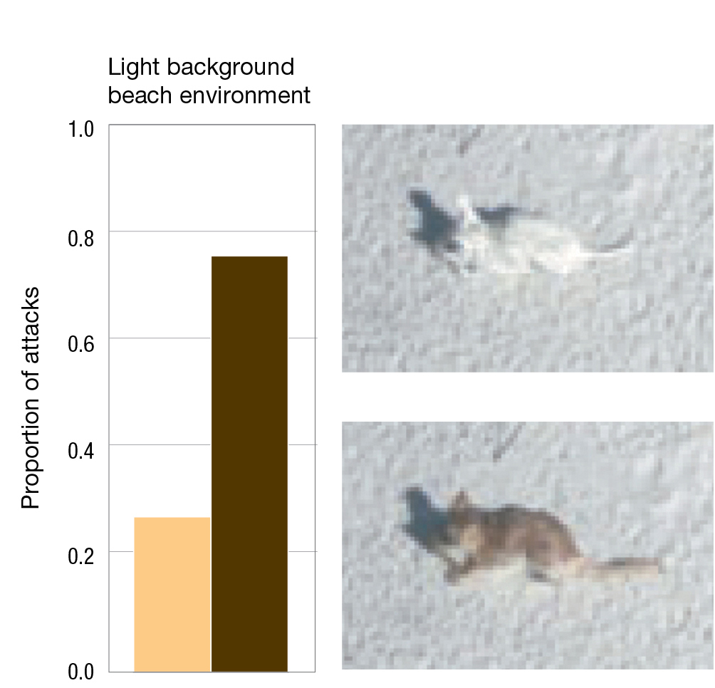
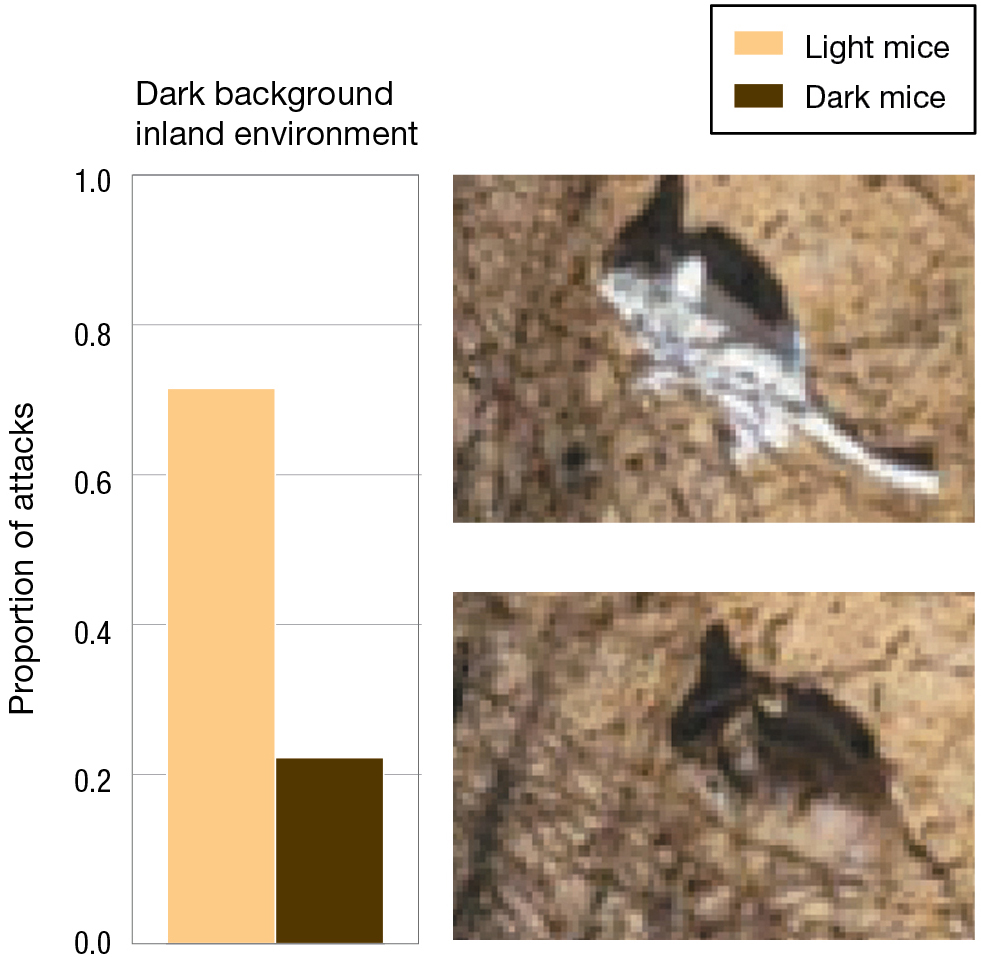
Many years later, in a follow-up to the Kaufman experiment, Hoekstra and her colleagues constructed silicone models that they painted to mimic either the dark- or light-coated oldfield mice, and they placed 125 models of each type in the natural environment of light sandy beaches or darker inland habitats (Vignieri et al. 2010). By using silicone models, Hoekstra and her team were able to remove a possible confounding variable that was present in the Kaufman experiment. In that earlier experiment, it is possible that different colored mice behaved differently, and that behavioral differences were responsible for differences in survival. Using silicone models eliminates this possibility. Attacks by predators could easily be detected by looking at the presence or absence of the silicone models over time, as well as marks from teeth, talons, or beaks on models that were not removed from a site by predators. The data from attacks provide strong evidence for a fitness advantage to mice that matched the color of their environment (Figure 3.8).
A
More information
A bar graph shows the proportion of attacks on mice in a light background beach environment with photos of the scenarios. Light mice are 0.27 and dark mice are 0.73. Photos of a white mouse and a brown mouse on light soil. The white mouse blends in more.
B
More information
A bar graph shows the proportion of attacks on mice in a dark background beach environment with photos of the scenarios. Light mice are 0.7 and dark mice are 0.21. Photos of a white mouse and a brown mouse on brown soil. The brown mouse blends in more.
FIGURE 3.8Predation, coat color, and fitness in the oldfield mouse using plastic models in the field. Hoekstra and colleagues placed light and dark silicone mouse models in light and dark environments to test predation rates. (A) Proportion of attacks against light and dark mice in the light environment. (B) Proportion of attacks against light and dark mice in the dark environment. Adapted from Vignieri et al. (2010).
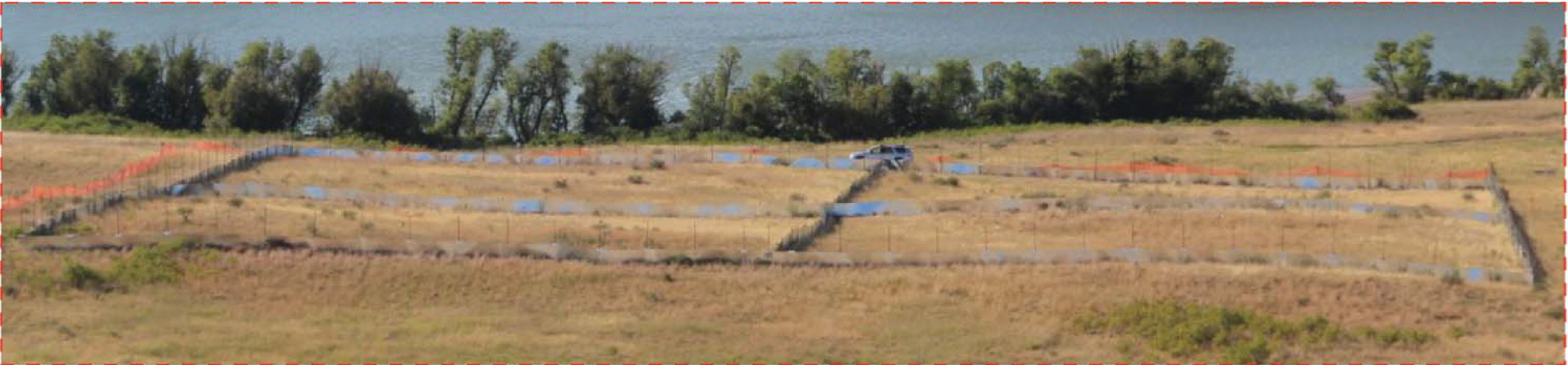
Ronan Barrett, Hoekstra, and colleagues have run a similar study of fitness in deer mice (Barrett et al. 2019). Deer mice, like oldfield mice, tend to have darker fur in habitats with dark vegetation and lighter fur in sand dune environments. Barrett et al. constructed large (50 meter × 50 meter) enclosures in both types of environments and removed mice and terrestrial predators from them. They then released individuals from the darker colored population into the enclosures in the sand dunes, and lighter colored individuals into the enclosures in the habitats with darker vegetation. As with the oldfield mice, individuals that were “mismatched” in terms of coat color and habitat suffered high predation rates (Figure 3.9).
A
More information
In an open field by a body of water, a large square enclosure has been set up. It is divided into four smaller enclosures.
B
More information
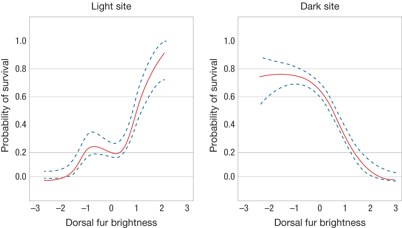
Two graphs relate dorsal fur brightness on the horizontal axis to probability of survival on the vertical axis. In the light site, brighter dorsal fur is associated with increased survival probability. In the dark site, brighter dorsal fur is associated with decreased survival probability.
FIGURE 3.9Coat color and fitness in the deer mice.(A) A 50 meter × 50 meter enclosure was built to measure the effect of coat color and fitness in a semi-natural environment (note the truck in the background for scale). These enclosures were at a sand dune site where deer mice have light color. Other enclosures were constructed where deer mice live in an environment with dark vegetation. (B) Probability of survival as a function of the brightness of dorsal fur in enclosures at both the sand dune and dark vegetation sites. The solid curve represents a curve of best fit and dashed lines represent plus or minus standard error.
Keep in mind that even small differences in fitness can translate into large changes in allele frequencies over time. For example, suppose that individual mice whose coat colors matched their environments produced just 1% more offspring per generation than those whose coat colors did not. Mathematical models show that over evolutionary time, this small difference could result in a population composed completely of individuals matching their backgrounds (we delve more into these mathematical models in Chapter 7). In a basic model with a few simple assumptions, the frequency of a gene associated with 1% more offspring per generation would double every 70 generations. In a population of 10,000 individuals, this gene variant could easily increase from a single copy to a frequency of 100% in a few thousand generations: a blink of the eye on an evolutionary timescale.
Natural selection appears to operate very strongly in both oldfield mouse and deer mouse populations. Indeed, we say that coat color in the oldfield mouse example is an adaptation. Let us now examine adaptations in greater detail.
KEYCONCEPT QUESTION
3.1 Thus far we have focused on genes as the means by which information is transferred across generations. This is only one way that such a transfer of information can occur. Cultural transmission is another. Examples of culturally transmitted information in humans include farming practices, musical tunes, fashions in clothing, and architectural techniques. Explain how a process analogous to natural selection might operate when culture is the means by which information is transferred from one generation to another.
The difference in the expected number of surviving offspring that can be attributed to having one particular genotype or phenotype instead of another. This is one component of natural selection.