3.4Natural Selection in the Laboratory

We have considered several examples of how evolutionary biologists generate and test hypotheses on natural selection in the wild. Biologists can do the same when it comes to natural selection in the laboratory. In one long-running experimental evolution study, researchers have even been able to do the following:

Watch as tens of thousands of generations of evolution take place.
Manipulate the physical environment to control nutrient availability, temperature, spatial structure, and other features, and manipulate the biotic environment, adding or removing competitors, predators, and parasites.
Create multiple parallel experiments with the same starting conditions in which to watch evolution unfold in replicate “universes.”
Move organisms around in a “time machine” so that they can interact with—and compete against—their ancestors or their descendants.
Go back in time to rerun evolution from any point, under the same or different environmental conditions.
Measure both allele frequencies and fitnesses to accuracies of 0.1% or less.

Let’s see how.

E. coli: Long-Term Evolution Experiment

Richard Lenski and his colleagues have been tracking evolutionary change for more than 75,000 generations in the bacterium Escherichia coli (Good et al. 2017; Lenski 2017). In 2022, at generation 75,000, this study, known as the long term evolution experiment (LTEE), moved to the laboratory of Jeffrey Barrett, a former postdoctoral researcher in the Lenksi lab. E. coli reproduces rapidly, dividing at rates upward of once per hour under favorable environmental conditions. As a result, Lenski and his colleagues have been able to observe evolution occurring in real time. To put 75,000 generations of bacterial evolution they have observed into perspective, the long term evolution evolution experiment now encompasses several times as many generations as there have been in the entire history of our species, Homo sapiens.

In 1988, starting with a genetically homogeneous strain of E. coli bacteria, Lenski created 12 parallel experimental lines—the original colonists of 12 parallel “universes.” The genotypes of each line differed only by an unselected marker gene that allowed researchers to keep track of which line was which. All 12 lines are kept in identical experimental conditions, but the lines are never mixed with one another. Instead, every day, Lenski and his team transfer cells from each of the 12 lines into fresh growth medium. Overnight, these cells go through six to seven generations of replication, and the next day the process starts anew. Periodically, a sample of the cells from each line is preserved in a –80°C freezer. This freezer serves as a “time machine”: Researchers thaw those cells at any point and can let them compete with their descendants (Figure 3.15). They can even use them to “start over” and can thus replicate the experiment from any point in time.

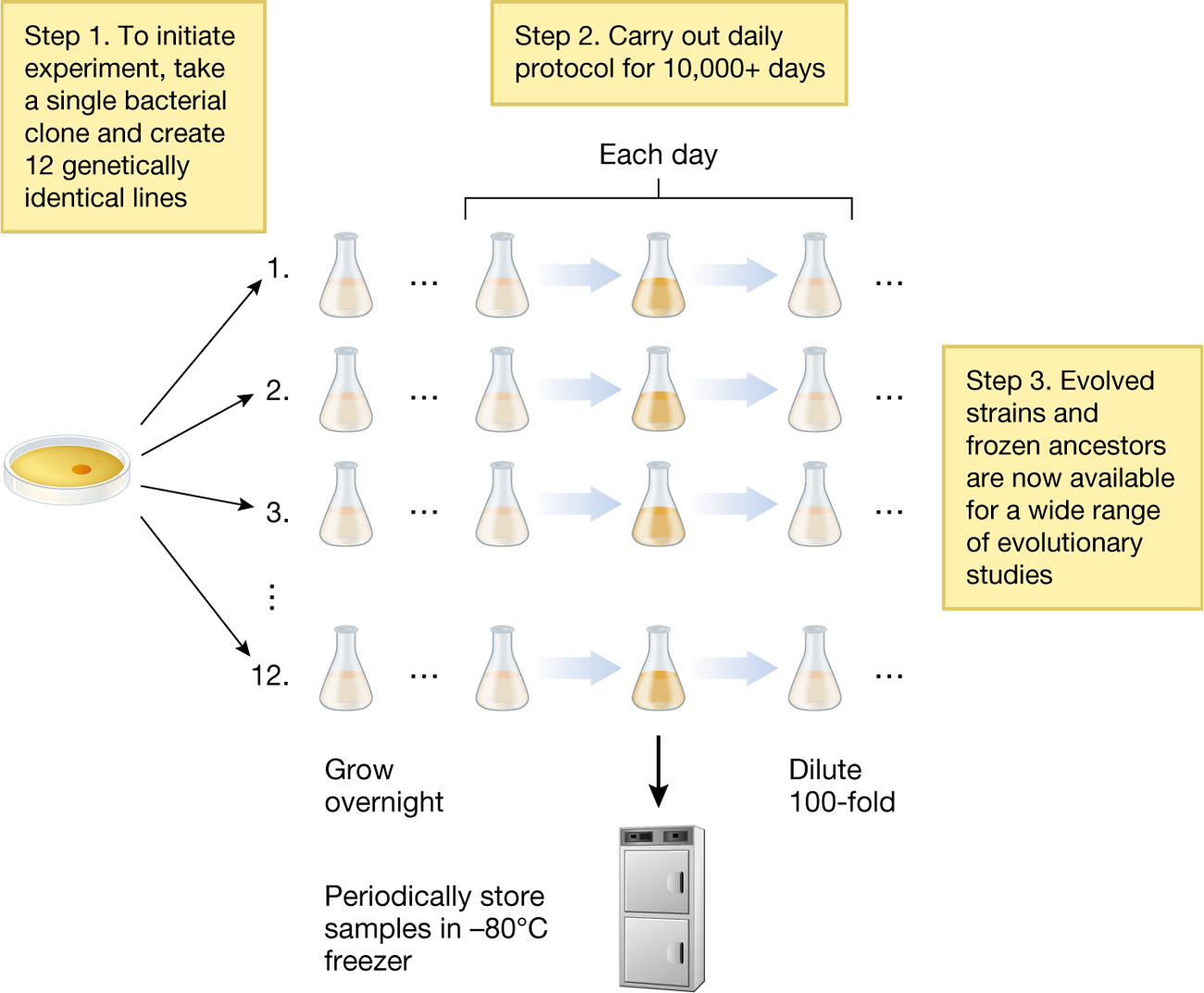
A diagram showing Lenski’s experimental evolution system. — FIGURE 3.15 Lenski’s experimental evolution system. The basic protocol for the Lenski *E. coli* experiment. Each day, Lenski and his team transfer cells from the 12 lines into fresh growth medium. These cells go through six to seven generations of replication overnight, and the next day the process starts anew. Periodically, the team freezes a sample of the cells from each line in a –80°C freezer. This open-ended system allows for a large number of potential experiments.

Evolutionary Change: Predictability and Quirks

So what can you do with an experimental system like this? We only know about one history of life: the one that actually took place on Earth and of which we are a living part. One question that has always fascinated evolutionary biologists is, what if you could “run the evolutionary process over again?” (Blount et al. 2018). Would the same phenotypes evolve the second time around? Or would we see something completely different? And if the same phenotypes did evolve, would the same underlying genetic changes be responsible or would natural selection find a different genetic path to a similar phenotypic outcome?

Early on in the long term evolution experiment, Lenski and his colleague Michael Travisano set out to address these questions by comparing what happened in the 12 replicate E. coli lines—the 12 parallel runs of evolutionary history (Lenski and Travisano 1994). To do so, they looked at a trait that evolved rapidly early in their experiment: the physical size of the individual E. coli cells. As Figure 3.16A illustrates, the average cell volume increased substantially over the first 2,000 to 3,000 generations of the experiment.

In the course of their experiment, the researchers removed a sample of E. coli cells after every 500 generations and then stored them in a freezer. By comparing cells sampled at different time points, the researchers could measure how fitness changed over time. Figure 3.16B shows what they found: the fitness of E. coli cells did indeed increase over the course of the experiment. Only 500 generations into the experiment, natural selection had already increased the fitness of the evolved strains relative to their ancestors, and this fitness difference continued to accumulate as the experiment progressed and more generations elapsed.

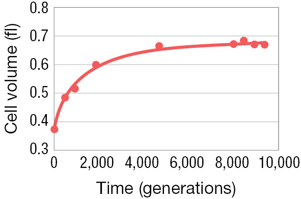
A line graph shows the change in volume of the E coli cell over time. — FIGURE 3.16 Cell size and fitness in one *E. coli* line. **(A)** Change in average cell volume (fl = femtoliter) in one of the 12 long-term lines. **(B)** Change in fitness for the same line, relative to its ancestor. Fitness values greater than one indicate higher fitness than the ancestor. From Lenski and Travisano (1994).

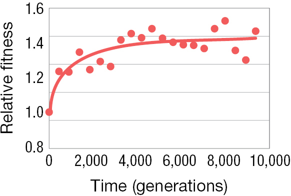
A line graph shows the relative fitness of the cell over time. — FIGURE 3.16 Cell size and fitness in one *E. coli* line. **(A)** Change in average cell volume (fl = femtoliter) in one of the 12 long-term lines. **(B)** Change in fitness for the same line, relative to its ancestor. Fitness values greater than one indicate higher fitness than the ancestor. From Lenski and Travisano (1994).

Figure 3.16 shows results from just one of the 12 lines, and in this line, cell size increased and fitness increased with it. Was this outcome a quirk of fate? What would happen if we were to replay the tape? Would cell size increase again? Lenski and Travisano were able to test this question directly by looking at the other 11 lines, each of which was an independent evolutionary run (Lenski and Travisano 1994). They found that in these lines, as in the first line, cell size invariably increased, and fitness of the cells increased relative to ancestral cells (Figure 3.17).

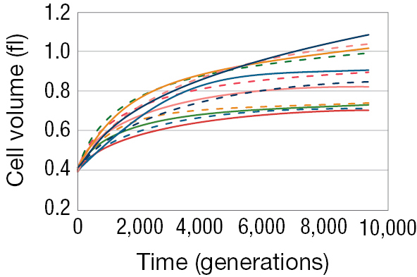
A line graph showing the cell size of 12 E coli lines. — FIGURE 3.17 Cell size and fitness in 12 *E. coli* lines. Change in **(A)** cell volume (fl = femtoliter) and **(B)** relative fitness in each of the 12 lines. Fitness values greater than one indicate higher fitness than the ancestor. From Lenski and Travisano (1994).

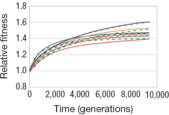
A line graph showing the relative fitness of 12 E coli lines over time. — FIGURE 3.17 Cell size and fitness in 12 *E. coli* lines. Change in **(A)** cell volume (fl = femtoliter) and **(B)** relative fitness in each of the 12 lines. Fitness values greater than one indicate higher fitness than the ancestor. From Lenski and Travisano (1994).

Phenotypically, the populations evolved in a similar fashion. Cell size always increased. But notice that despite starting with genetically identical cells and subjecting them to identical environments, cell size increased more in some lineages than in others. Natural selection operated in a similar direction in each case, but it appears not to have taken an identical path. Likewise, fitness increased in every one of the 12 lines, but some of the lines seem to have found better paths than others, and there was considerable variation in fitness between the lines after 10,000 generations. These results highlight that evolution by natural selection is in some aspects a predictable, repeatable process—and yet it is also one in which random events, such as which mutations occur or the order in which they occur, can play a significant role in shaping the course of history.

Over the past 30 years, Lenski and his colleagues have studied numerous other traits in these 12 bacterial lines, and in doing so, they have tested many evolutionary hypotheses. In the next subsection, we will look at a thermal adaptation experiment that Lenski and colleagues used to test another question in evolutionary biology: What are the constraints on what natural selection can achieve? Why are organisms not perfectly adapted to all environmental conditions?

Thermal Adaptation and Antagonistic Pleiotropy in E. coli

Let a bacterial population evolve for a few hundred generations under any particular set of laboratory conditions, and fitness under those conditions will tend to increase significantly. Yet Lenski and his team found that E. coli lines grown at a steady temperature of 37°C—which is right in the middle of the 35–40°C range of temperatures that E. coli experiences in the guts of their typical hosts—were able to evolve to grow even more effectively at that temperature over the course of their experiment. What is going on here? Why should fitness have increased in this experiment? After all, before Lenski ever began his experiments, E. coli had already undergone many billions of generations of adaptive evolution in which they might have evolved higher fitness at around 37°C. Why hadn’t these organisms already done so?

One possibility is that there are trade-offs between an organism’s ability to perform under one set of environmental conditions and its ability to perform under another. Perhaps E. coli cells are not optimized for growth around 37°C because, unlike the controlled temperature conditions they experienced in Lenski’s laboratory, they normally experience other temperatures as well—and adaptations that increase fitness at 37°C may decrease fitness at those other temperatures. To address this hypothesis, Lenski and his colleagues asked whether evolutionary changes that increase growth rate at one specific temperature will be associated with a reduction in growth rates at other temperatures (Huey and Hertz 1984; Palaima 2007).

The growth rates of E. coli cells from generations 2,000, 5,000, 10,000, 15,000, and 20,000 were each compared to the original population of cells, and this comparison of growth rates was repeated across an array of nine temperatures from 20°C to 42°C in all 12 of Lenski’s E. coli universes (Cooper et al. 2001) (Figure 3.18). After 20,000 generations in an environment where the temperature was 37°C, natural selection led to an increase in growth rate at that temperature. Moreover, the optimal temperature for growth shifted from approximately 40°C to near 37°C. Lenski and his team also found an evolutionary change toward lower growth rates at both extremes of the temperature range—20°C and 42°C—in the majority of populations that evolved optimal performance at 37°C (Cooper et al. 2001; Bennett and Lenski 2007).

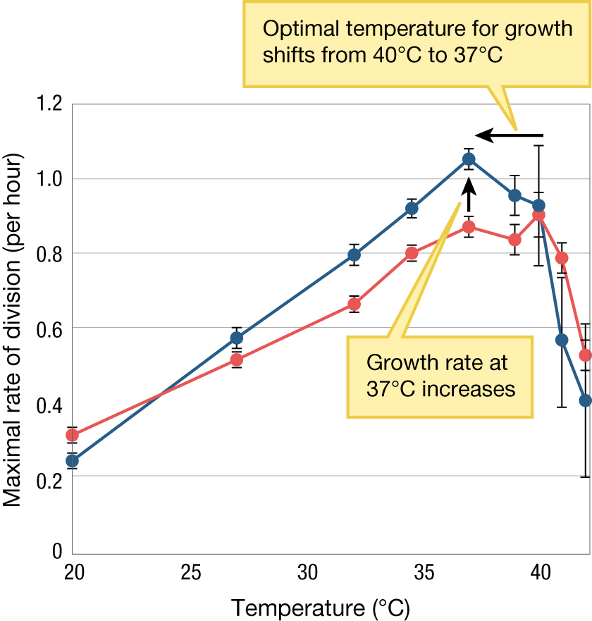
A line graph with plotted data showing thermal adaptation in E. coli. — FIGURE 3.18 Thermal adaptation in E. coli. The red line represents ancestral population, and the blue line represents the population after 20,000 generations at 37°C. Adapted from Cooper et al. (2001).

Why did this happen? Why did evolving an optimal performance at 37°C lead to suboptimal results at the other temperatures (20°C and 42°C)? One possibility is a nonselective explanation: Perhaps after growing for 20,000 generations at 37°C, Lenski’s lines had accumulated mutations that reduced their ability to grow at 20°C or 42°C. Because the bacteria were never exposed to those temperatures, natural selection would not have acted against such mutations. But Cooper and his colleagues were able to find evidence against this hypothesis in a clever way. Among their 12 lines, 3 lines evolved to become so-called mutator strains, with much higher mutation rates than those observed in the other 9 lines. If the decline in performance at 20°C and 42°C had resulted from the accumulation of unselected mutations, Cooper and his team reasoned, the decline in performance should be greater in the mutator strains, because these strains accumulated far more mutations. But they found no such difference. Simple mutation accumulation seems an unlikely explanation for the fitness decline at the extreme temperatures.

Instead, Lenski and his colleagues suggest that their results are best explained by a phenomenon known as antagonistic pleiotropy. The antagonistic pleiotropy hypothesis proposes that the same gene (or genes) that codes for beneficial effects—here, rapid growth at 37°C—also codes for deleterious effects in other contexts; in this case, poor performance at 20°C and 42°C. When genes, such as those hypothesized here, affect more than one characteristic, they are referred to as pleiotropic genes. And because we are testing whether such pleiotropic genes have a negative effect in one context but a positive effect in another, we refer to this as antagonistic pleiotropy. Thus, antagonistic pleiotropy results in a trade-off between fitness under one set of conditions and fitness under another set of conditions.

One prediction from the antagonistic pleiotropy hypothesis is that the negative components to fitness—in this case, poor performance at 20°C to 42°C—should build up quickly and early in the tested populations because variation in response to temperature will be high at the start of the process, and hence selection for optimal performance will be most powerful. The experimental results provide support for the antagonistic pleiotropy hypothesis because suboptimal performance at extreme temperatures evolved fairly quickly in their populations, with most selection occurring in the first 5,000 of the 20,000 generations of Lenski’s laboratory populations of E. coli.

Lenski and his team conducted a follow-up experiment on the effect of temperature that sheds light on the process of convergent evolution. They began with a single population that had recently gone through 2,000 generations growing in an environment where the temperature was 37°C. From this culture, they created 30 populations, made up of six replicate populations in each of five temperature regimes—a constant 20°C, 32°C, 37°C, or 42°C and one treatment that on alternate days experienced 32°C or 42°C. These 30 populations were allowed to grow and evolve for an additional 2,000 generations (Deatherage et al. 2017). They then sequenced the genome of one representative sample from each of the 30 populations and compared it to the genome of individuals in the original culture and to each other. They examined mutations that had built up in the genome over the course of 2,000 generations, targeting mutations that unambiguously affected a single gene. Figure 3.19 compares the percentage of mutations shared in common among populations evolved at the same temperature with the percentage of mutations in common among populations evolved at different temperatures. The data show that first, populations evolved at the same temperature share more mutations than populations evolved at different temperatures. Even among populations evolved at the same temperature, shared mutations are in the minority. Exactly how these new genes affect survival as a function of temperature is still not clear, although Lenski and his team have identified a number of candidate genes that may be important in adaptation to temperature.

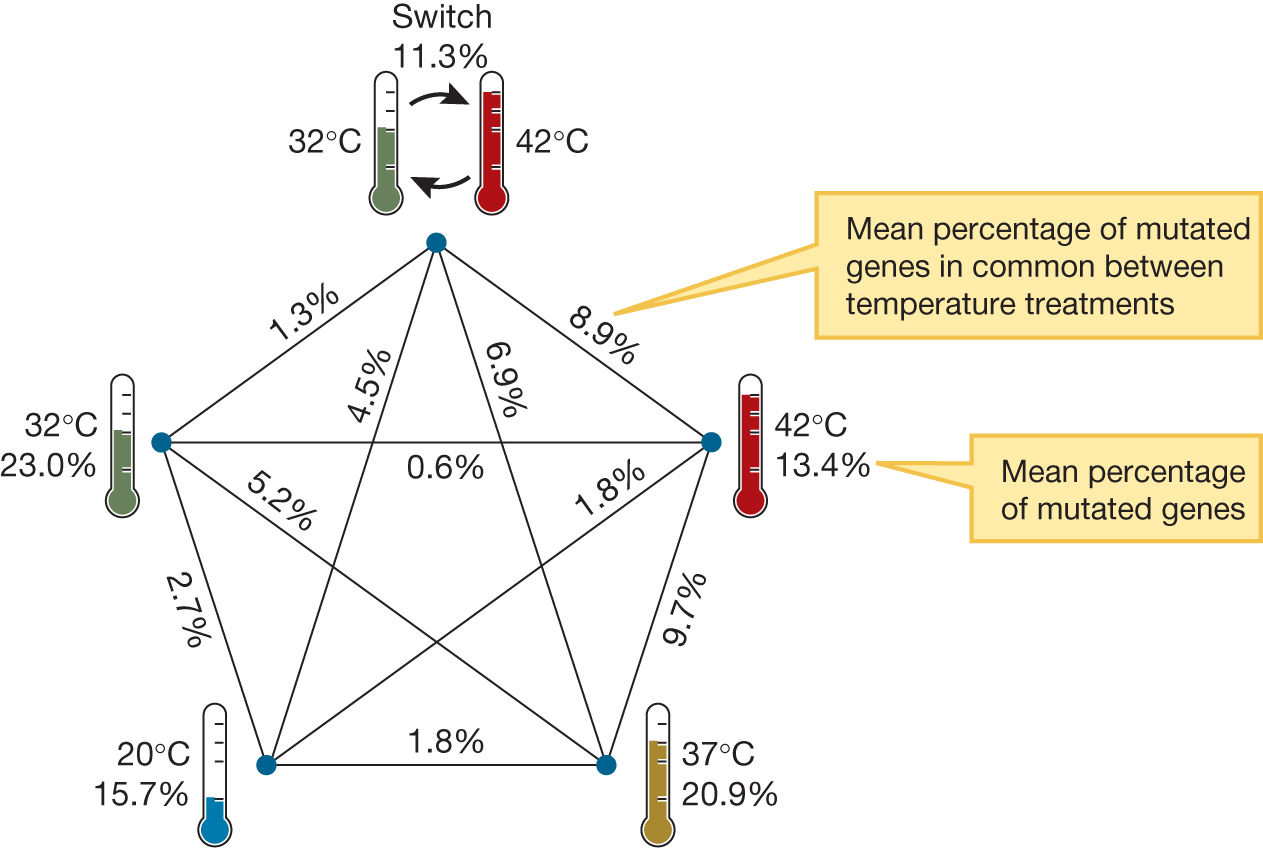
Genetic similarities and differences among five different temperature regimes. — FIGURE 3.19 Similarities and differences between temperature regimes. Each vertex of the diagram represents one specific temperature regime. Lines between vertices are labeled with similarity scores indicating the mean percentage of mutated genes (S_w) that these regimes have in common. The percentages listed adjacent to the thermometer icons show the mean percentage of mutated genes (S_b) in common across the six populations for a given temperature regime. The difference between S_b and S_w was used as a measure of temperature-specific pattern of genomic evolution. All pairs except the “alternating between 32°C and 42°C” and 42°C were significantly more similar within runs of the same condition compared to between runs of different conditions. This indicates convergent evolution among the replicate lineages run at each temperature.

KEYCONCEPT QUESTION

3.3 How might the antagonistic pleiotropy hypothesis be related to diseases that are often associated with old age (for example, Alzheimer’s disease)?

marker gene: A neutral gene with readily observable phenotypic consequences that can be used to track different experimental lines.
antagonistic pleiotropy: A phenomenon in which a single gene has multiple phenotypic consequences with opposing effects on fitness. See also pleiotropic genes.
pleiotropic genes: Genes that affect more than a single trait.

3.4Natural Selection in the Laboratory

E. coli: Long-Term Evolution Experiment

Evolutionary Change: Predictability and Quirks

Thermal Adaptation and Antagonistic Pleiotropy in E. coli

Glossary