3.6Constraints on What Natural Selection Can Achieve
In our efforts to understand the process of natural selection, it is critical to recognize the limitations on what natural selection can achieve. In the short term, there may be limits on the genetic variation available for natural selection to operate on (Futuyma 2010). Constraints on what natural selection can achieve have been examined experimentally many times by evolutionary biologists, including in another set of E. coli experiments conducted by Lenski and his team. They found that under certain conditions, the rate of adaptation in E. coli was proportional to the supply of new variation available (de Visser et al. 1999).
Even if there is variation in a given characteristic, selection may be unable to act on that characteristic if the genes involved have effects on other characteristics that are also under selection. Another short-term constraint on natural selection is that the influx of genes into a local population can limit the degree of local adaptation; that is, a peripheral population may be unable to adapt to its local environmental circumstances because of the continual influx of genes from a larger population that faces different selective conditions.
In the long term (assuming that extinction does not occur), these limitations may be overcome. Even in small populations, mutations that overcome some constraint may eventually appear; it may simply be a matter of time. Correlated characteristics may become uncoupled once the appropriate mutations arise, removing the constraints associated with pleiotropy. Reproductive isolating mechanisms can reduce or eliminate gene flow into the peripheral population and thus allow local adaptation. Still, in the long term, there are other limitations to what the process of natural selection can achieve. First we will look at some of these limitations, then we will look at how, in some cases, they may be overcome.
Physical Constraints
From a spider’s web, with its minuscule weight and exceptional tensile strength, to an owl’s fringed feather edges that muffle any sound from its wings as they cut through the air, natural selection has fashioned countless material marvels. Nonetheless, natural selection is limited in what it can do. It operates on physical structures in the material world, and as such it is constrained by the same physical and mechanical laws that limit the realm of possibility for human engineers.
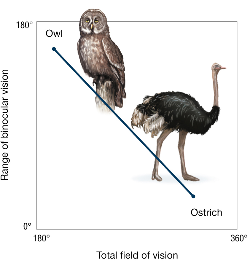
Compare the placement of the eyes in an ostrich to that in an owl (Figure 3.29). The ostrich—which must remain vigilant against predators—has eyes that are set on either side of the head, allowing a nearly 360° field of view, but affording almost no stereoscopic vision because the field of each eye scarcely overlaps with that of the other. The owl—a visual predator—has eyes that are set on the front of the head, allowing a fully stereoscopic view of its environment, including prey species, but presenting a much more limited field of view than that enjoyed by the ostrich.
More information
The line graph shows the trade-offs in binocular vision in an owl and an ostrich. The x axis is labeled with total field of vision and the y axis is labeled with range of binocular vision. The line of the graph is a negative linear slope with the owl at the top left hand corner and the ostrich at the lower left hand corner. The owl has a range of binocular vision of 180 degrees, but its total field of vision is very limited. The ostrich has a total field of vision of 360 degrees, but its binocular vision is very limited.
More information
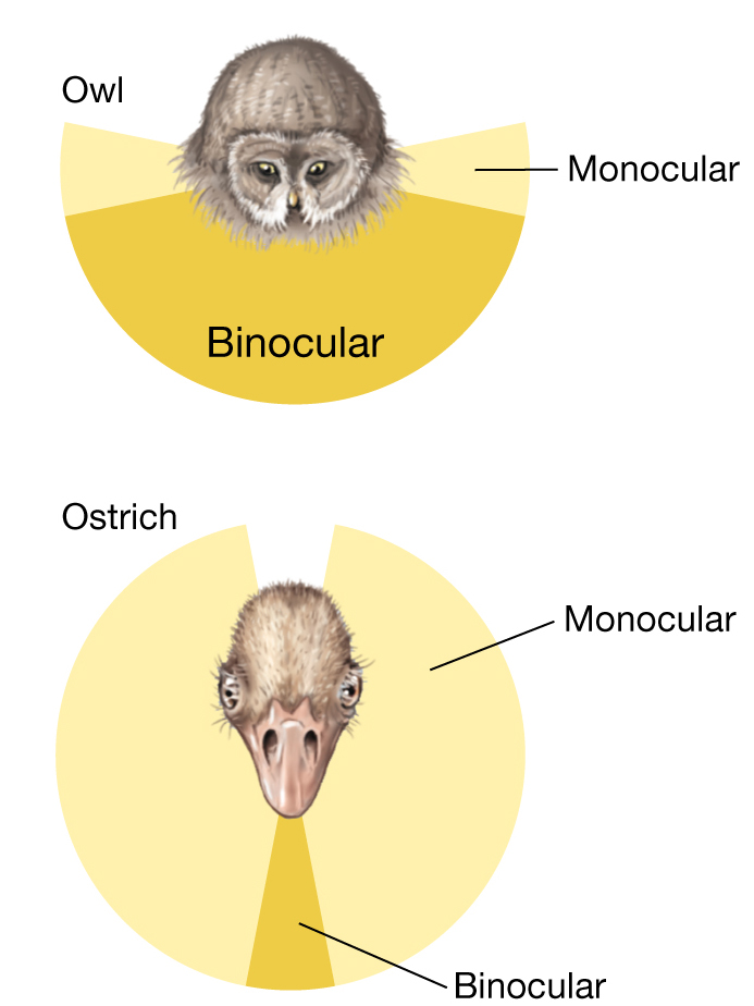
A diagram showing the trade-offs in binocular vision between an owl and an ostrich. The position of the eyes determines where along the trade-off curve a species falls. The owl’s eyes are in the front side by side, making its binocular view greater than its monocular view. The ostrich’s eyes are on the side of its head, limiting its binocular view but making its monocular view greater.
More information
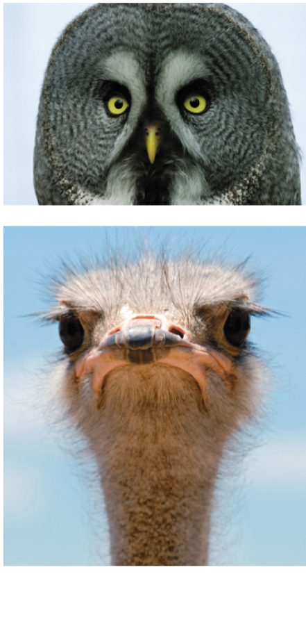
Photos comparing the eyes of a great gray owl and an ostrich. The owl’s eyes are close together on the front of the head. The ostrich’s eyes are far apart toward the sides of the head.
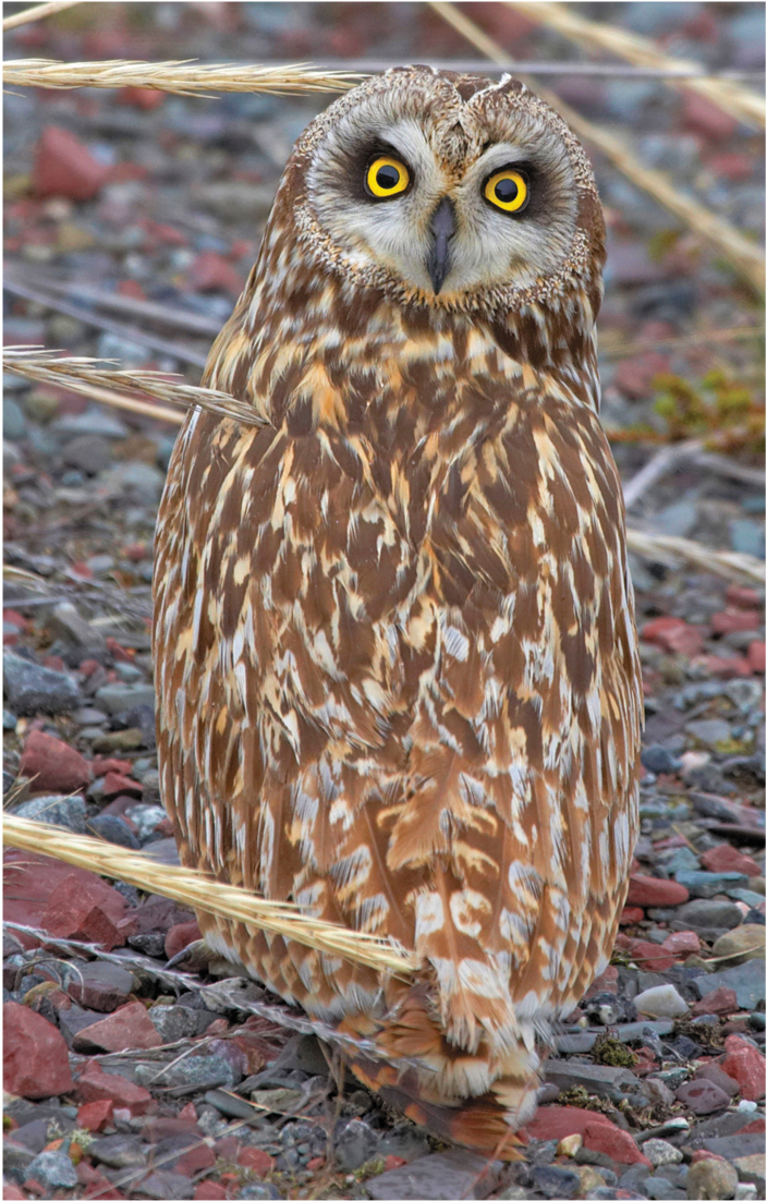
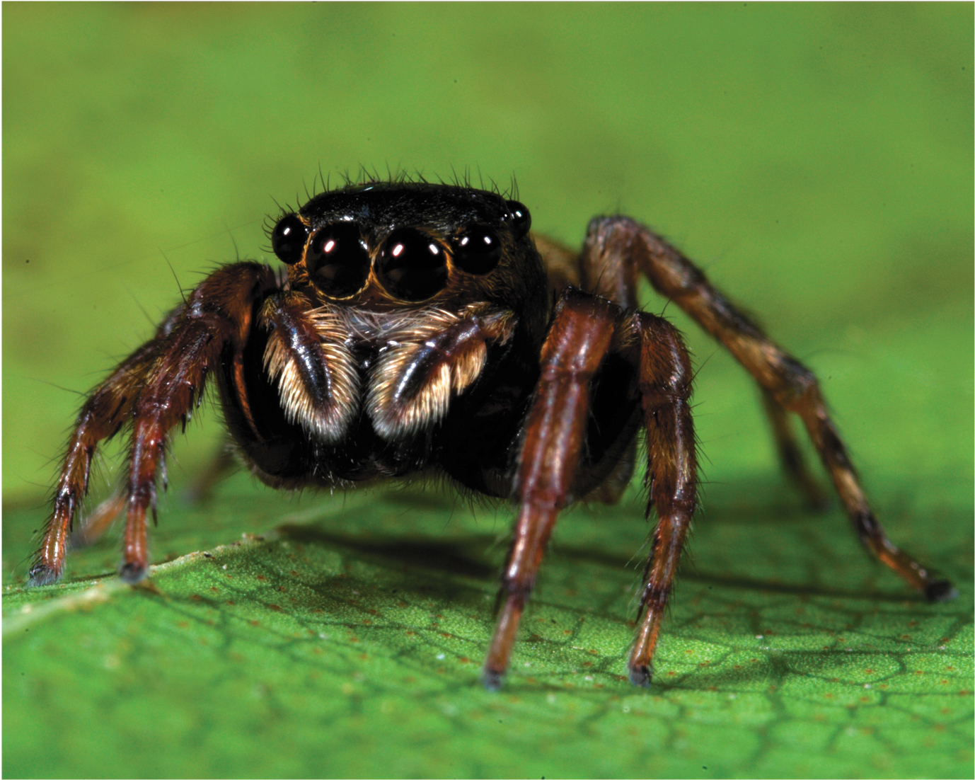
The ostrich and the owl represent two extreme manifestations of the response to the constraint that a two-eyed organism can have a 360° field of view or binocular vision across most of the visual field, but the laws of physics tell us they cannot have both. For their part, owls have evolved a partial solution to this constraint: An owl can turn its neck nearly 180° over its back without shifting its perch (Figure 3.30A). Spiders go a step further. They have eight eyes, allowing them to see in 360° and at the same time to enjoy a binocular (or even multiocular) forward view for visual hunting (Figure 3.30B).
More information
An owl with his head turned 180 degrees.
More information
A jumping spider with many front-facing eyes sitting on the surface of a leaf.
Other simple physical constraints become apparent when we look at the sizes and shapes of animals (Thompson 1917; Haldane 1928; Gould 1974). Why are there no insects that are the size of wolves? Why don’t single-celled swimmers have the same streamlined shape that we see in dolphins, tuna, or penguins? Why are there no elephant-sized creatures with spindly spiderlike legs?
More information
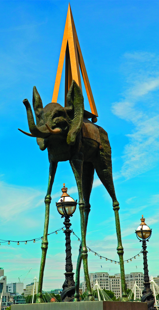
A sculpture by Salvador Dali called the Space Elephant. The elephant has long thin legs like stilts and carries a large triangular structure on its back.
The answer to each of these questions lies in the constraints that the laws of physics place on the form and structure of living organisms. As an example, let us consider in detail the last of these questions—why are there no elephant-sized creatures with spindly spiderlike legs? When we look at Salvador Dali’s sculpture Space Elephant, our intuition about the world tells us that this creature is absurd (Figure 3.31). Why? At least for elephant-sized creatures made of flesh and blood, it seems as if legs like that would be too fragile to support the immense bulk of the body held high above.
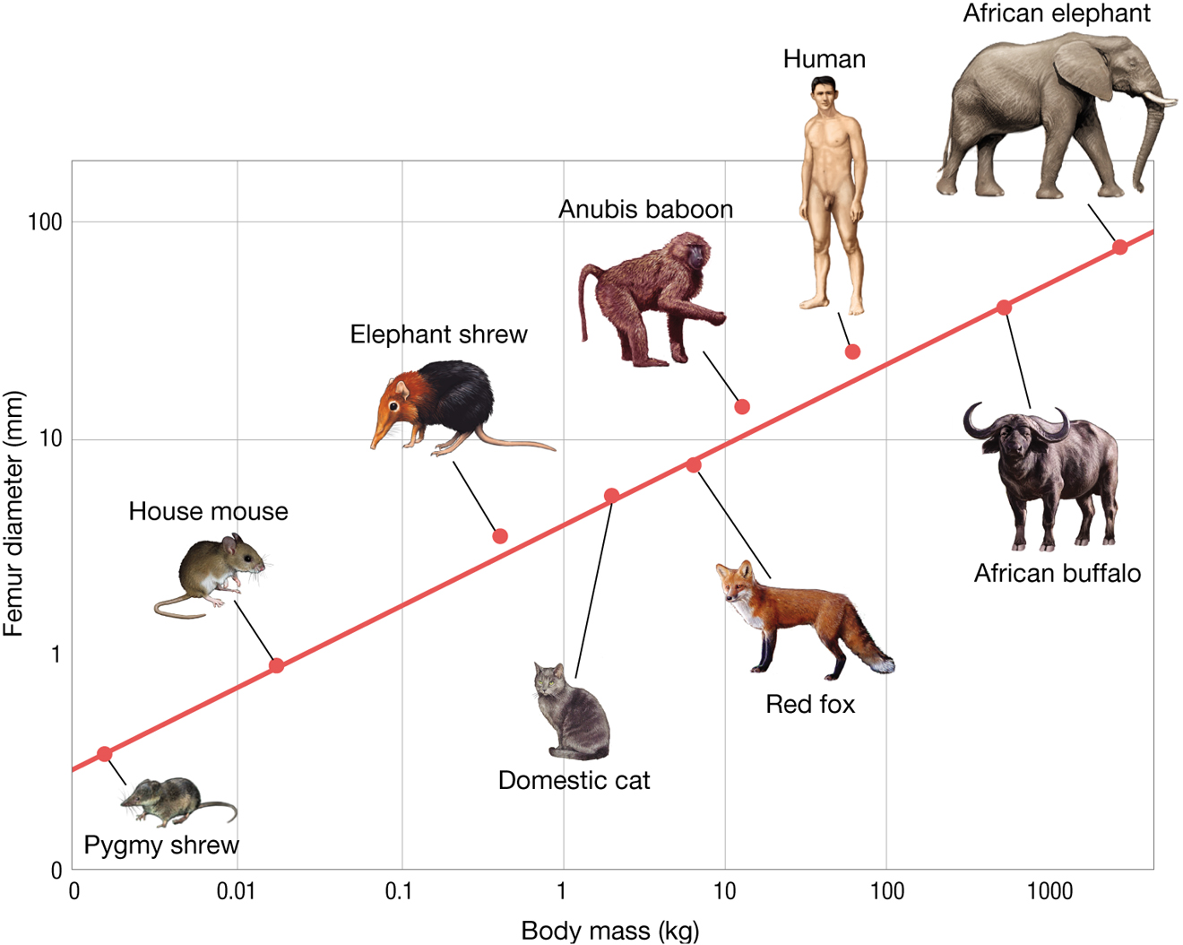
Indeed, if we look at leg size (diameter) relative to body mass, we see that mammals, from the tiny pygmy shrew to the massive African elephant, conform to a tightly defined relationship between body mass and leg diameter. Figure 3.32 plots the diameter of the femur against total body mass for different species of mammals (Alexander et al. 1979). All of the mammals measured lie along a tight line across a millionfold difference in body mass. Why is this? Why has natural selection not chosen some solutions somewhere off this line? Is it an accident of history or is there some physical constraint that shapes the relation between body mass and femur diameter?
More information
A line graph measuring femur size and body mass in different species. The x axis is labeled with body mass in kilograms that ranges from 0 to 10,000 kilograms, with each tick mark increasing ten-fold. The y axis is labeled with femur diameter in millimeters that ranges from 0 to 100 millimeters. The line on the graph is a positive linear slope. A pygmy shrew has a body mass of about 0.003 kilograms and a femur diameter of about 0.5 millimeters. A house mouse is about 0.02 kilograms and has a femur diameter of about 1 millimeter. An elephant shrew is about 0.7 kilograms and has a femur diameter of about 5 millimeters. A domestic cat is about 3 kilograms and has a femur diameter of about 7 millimeters. A red fox is about 8 kilograms and has a femur diameter of about 9 millimeters. An Anubis baboon is about 15 kilograms and has a femur diameter of about 15 millimeters. A human is about 80 kilograms and has a femur diameter of about 40 millimeters. An African buffalo is about 590 kilograms and the femur diameter is about 55 millimeters. An African elephant is about 5,000 kilograms and the femur diameter is about 90 millimeters.
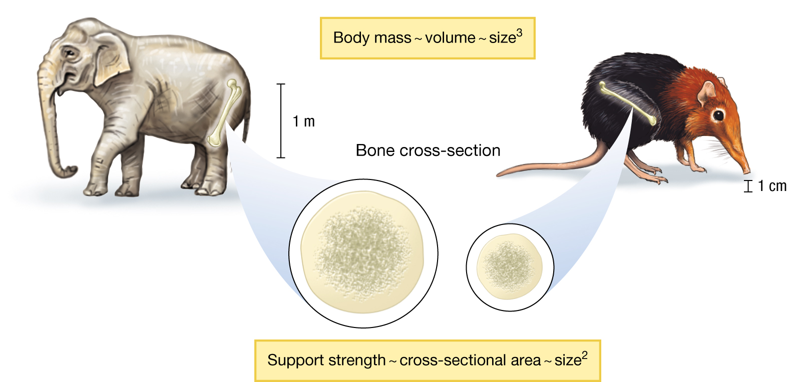
All else being equal, organisms with longer, thinner legs will be faster and lighter. So, perhaps we should not be surprised that there are no organisms with small bodies and thick legs. But why don’t we see the converse—organisms with large bodies and thin legs as illustrated by Dali? We can find the answer in the simple scaling laws of support structures, as illustrated in Figure 3.33. Looking at an ensemble of similarly shaped organisms, notice first that body mass increases with the third power of size (for example, measured as body length or height): mass ~ size3. But the strength (that is, the ability to resist compressional stress) of a supporting structure is proportional to its cross-sectional area, which scales with the second power of size: cross-sectional area ~ size2.
More information
An illustration of an elephant and an elephant shrew comparing their body mass and bone cross-sections. Body mass scales with the third power of size. The bone of an elephant leg is about 1 meter long and the bone of an elephant shrew is about 1 centimeter long. The support strength scales with the second power of size.
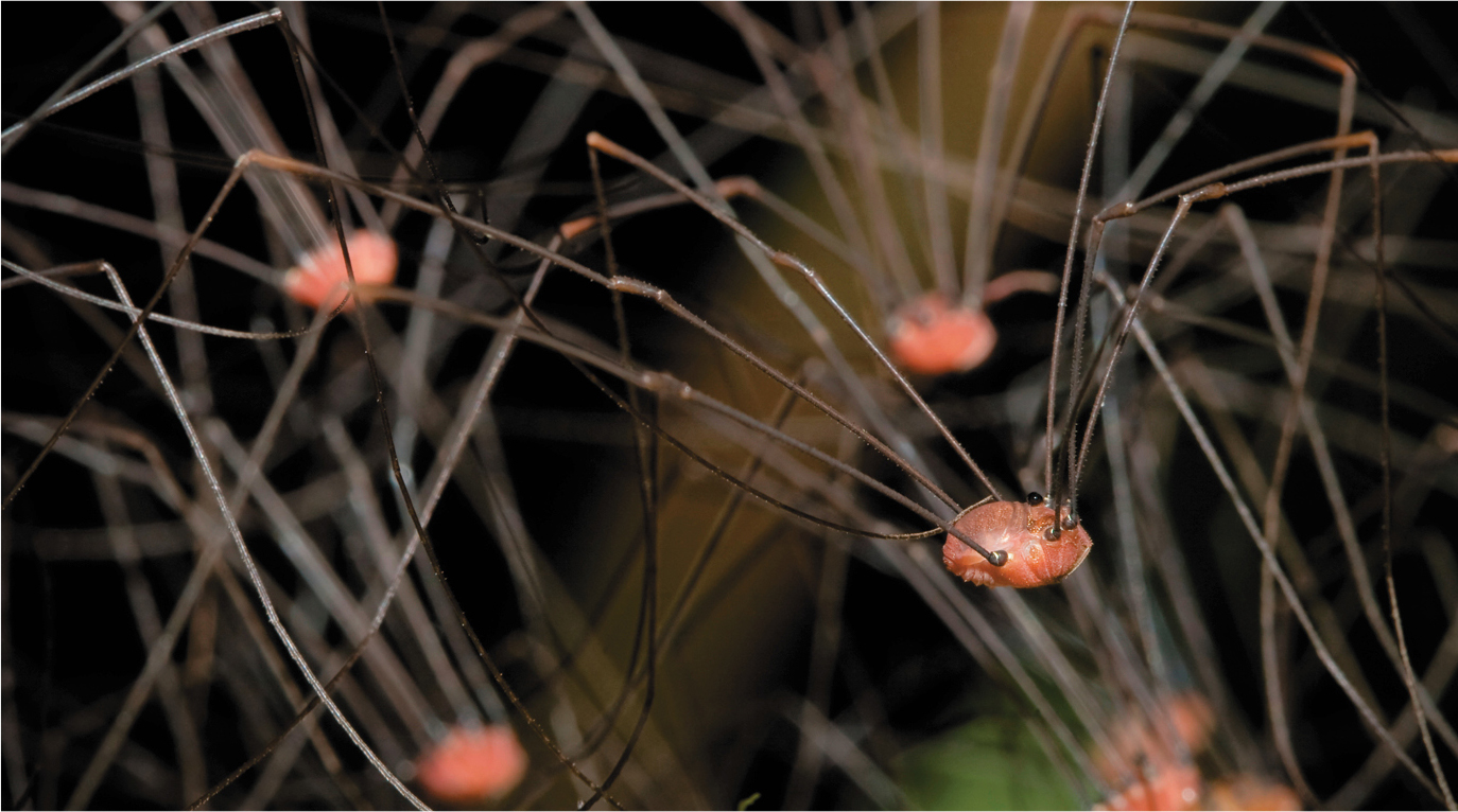
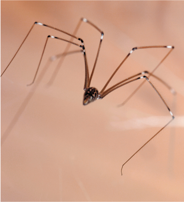
Because of this scaling relationship, legs must get proportionally thicker, relative to size, as an animal gets larger. Thus, it is not that we cannot have creatures with the relative proportions of Dali’s elephant; it is just impossible to have elephant-sized creatures of these proportions. The harvestman arachnids (sometimes called daddy longlegs) and Pholcus spiders provide examples of how, at tiny size scales, natural selection can produce creatures with a limb geometry akin to that of Dali’s elephant (Figure 3.34).
More information
A group of Harvestman spiders with red bodies and brown legs.
More information
A brown cellar spider.
Evolutionary Arms Races
Another important reason that organisms are not perfectly adapted to their surroundings is that their surroundings do not present a stationary “target” for natural selection to aim at to optimize phenotype. The abiotic environment changes over geological timescales: Ice ages come and go, oxygen concentrations rise and fall, continents shift, and temperatures fluctuate. Natural selection may produce organisms with adaptations to many of these slow changes, but there are faster changes in the abiotic environment as well. Conditions vary from season to season; some years are drier or wetter, hotter or colder than others. Changes in the biotic environment are even more important. Much of what is significant about an organism’s environment is provided by other organisms, which themselves are evolving by natural selection as well.
Let us look at a couple of examples in which evolutionary change in one species can affect selective conditions for a second species—a phenomenon known as coevolution (Chapter 18). As a case in point, why are all organisms vulnerable to infectious diseases? Why haven’t they evolved better defenses against pathogens? We will explore this question in further detail in Chapter 20, but let us now briefly consider just one of the major reasons: Organisms have not evolved impenetrable defenses against pathogens because pathogens are evolving, too. As a pathogen’s hosts evolve to deter or fight off infection more effectively, natural selection on the pathogen population intensifies, favoring variants that are able to elude the host’s defenses.
The simultaneous action of natural selection on each side of the host–pathogen interaction is known as an evolutionary arms race, analogous to the bilateral weapons buildup that characterized the Cold War between the United States and the former Soviet Union. Each side is continually selected for new weapons or new defenses that enable it to hold its own against the other.
We see a similar evolutionary arms race in the interaction between predators and prey. Prey are selected to become increasingly effective at escaping their predators; their predators in turn are selected to become increasingly good at capturing these ever-more-elusive prey. The prey is not always able to escape, and the predator is not always able to capture its mark because they are locked into a coevolutionary struggle. We will explore the coevolutionary process in detail in Chapter 18.
Natural Selection Lacks Foresight
Another reason that organisms are not perfectly adapted to their environments is that the process of natural selection lacks foresight. Natural selection has no way of anticipating the future beyond reacting to the past and the present, nor can it plan ahead by multiple steps. Selection favors changes that are immediately beneficial, not changes that may be useful at some time in the future. What this means is that if a new structure is to arise by natural selection alone, every step along the way must be favored.
To get a sense of just how difficult it can be to evolve major new structures by incremental changes, consider the following challenge. Suppose that we play a game in which we are given an old jalopy and a warehouse full of auto parts. Our goal is to convert the jalopy into a sleek and powerful race car—but there is a catch. Each time we swap even a single part on the car, the rules state that the car has to be in running condition. Worse yet, after each swap, we have to be able to drive the car around a racetrack faster than it could achieve prior to the swap. These requirements certainly restrict our options for how we do the work. We cannot, for example, strip the entire car down and change the whole transmission or the whole engine in one major overhaul. Instead, we have to find a path of gradual changes, switching single bolts and single belts and single pistons one by one, always improving the lap times, and eventually producing the race car.
Natural selection has to do something similar as body plans change and new structures evolve. Those evolutionary changes that arise by natural selection tend to make the organism more fit than it was before the changes took hold. And, of course, natural selection doesn’t have intentionality; it does not have a goal or target “in mind.” We could even say that, in the case of the race car, the player doesn’t know what the parts are or what they do. The player simply tinkers with the car, making little changes, keeping those that make the car faster, discarding those that do not.
Despite these difficulties, this problem is not insurmountable. There may be a sequence of single part swaps that enables the car to go from jalopy to race car, always reducing the lap times. Such swaps may require that some parts of the car change functions. For example, rather than fashioning a spoiler from scratch, we might build it out of another part of the car. Perhaps we might convert the lid of the trunk into a spoiler. Why not? Race cars don’t need a trunk for carrying luggage. Another possibility is that we might add new parts to the jalopy before removing old ones. We could add disc brakes before removing the current drum system. We could even add parts that we would later remove entirely; we could add structural supports to carry the car through some of the intermediate stages, and then remove them later to reduce weight.
Natural selection can move along a similar path on the way to evolving new structures. And, of course, natural selection is not the only evolutionary process operating; as we will see in later chapters, genetic drift, genetic hitchhiking, and many other mechanisms also play important roles in determining the direction of evolutionary change. Thus, new structures can arise from a combination of selective and nonselective processes.
We have seen how the process of natural selection requires three components—variation, heritability, and fitness differences. When a trait has been under natural selection for a specific function in a specific population, and that trait serves the same primary function or functions today as it did in the past, we call it an adaptation. Adaptations can be studied both in the wild, as we saw with oldfield mice, guppies, and anole lizards, and in the laboratory, as we discovered in our discussion of cell size and temperature sensitivity in E. coli. Through the use of studies that have ranged from the scale of the molecule to the whole organism, we have also explored various ways that the evolutionary process can lead to complex traits, such as the vertebrate eye and the aldosterone–M receptor pairing both through classic step-by-step adaptation for a specific function and through exaptation. We have also seen that constraints limit the power of selection.
We now shift our emphasis from natural selection and the adaptations it produces to phylogeny and common descent in Chapters 4 and 5.
Glossary
- coevolution
- The process in which evolutionary changes to traits in species 1 drive changes to traits in species 2, which feed back to affect traits in species 1, and so on, back and forth, over evolutionary time.
- evolutionary arms race
- A form of coevolution in which the species involved each evolve countermeasures to the adaptations of the others; most often associated with host–pathogen and predator–prey coevolution.