3.5Well-Behaved Preferences

We’ve now seen some examples of indifference curves. As we’ve seen, many kinds of preferences, reasonable or unreasonable, can be described by these simple diagrams. But if we want to describe preferences in general, it will be convenient to focus on a few general shapes of indifference curves. In this section we will describe some more general assumptions that we will typically make about preferences and the implications of these assumptions for the shapes of the associated indifference curves. These assumptions are not the only possible ones; in some situations you might want to use different assumptions. But we will take them as the defining features for well-behaved indifference curves.

First we will typically assume that more is better, that is, that we are talking about goods, not bads. More precisely, if $(x_1,x_2)$ is a bundle of goods and $(y_1,y_2)$ is a bundle of goods with at least as much of both goods and more of one, then $(y_1,y_2)\succ (x_1,x_2)\text{.}$ This assumption is sometimes called monotonicity of preferences. As we suggested in our discussion of satiation, more is better would probably only hold up to a point. Thus the assumption of monotonicity is saying only that we are going to examine situations before that point is reached—before any satiation sets in—while more still is better. Economics would not be a very interesting subject in a world where everyone was satiated in their consumption of every good.

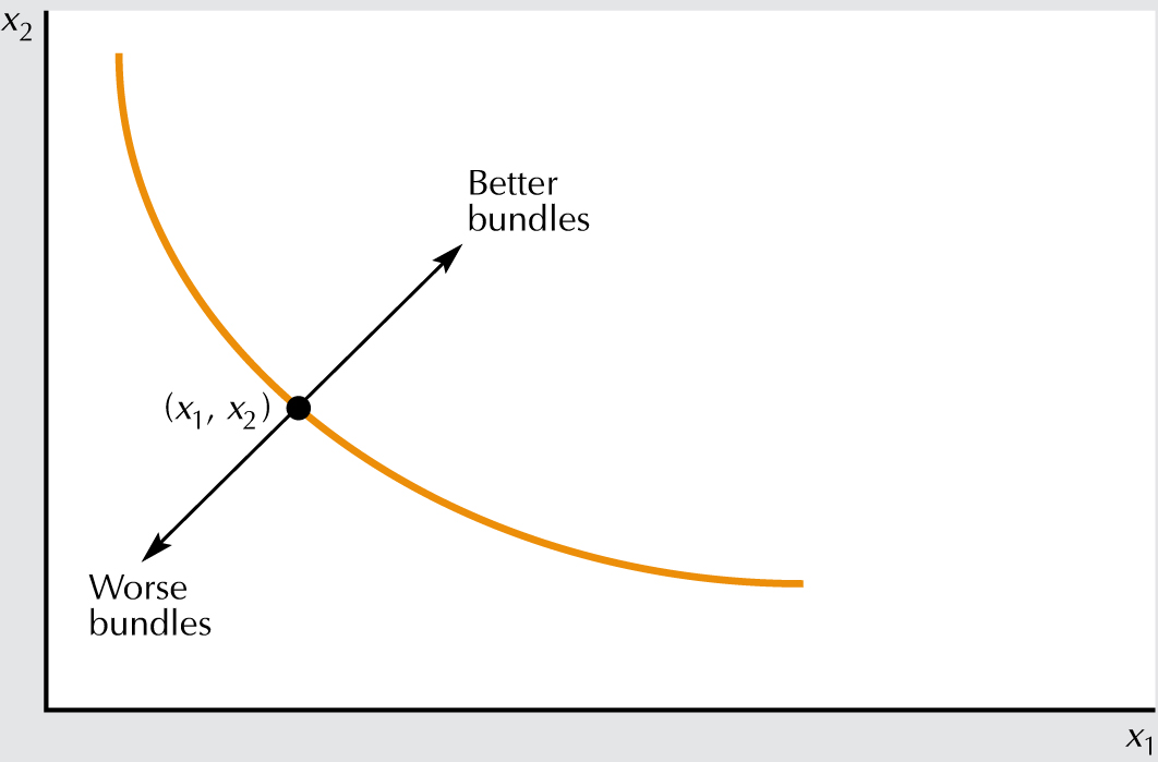
What does monotonicity imply about the shape of indifference curves? It implies that they have a negative slope. Consider Figure 3.9. If we start at a bundle $(x_1,x_2)$ and move anywhere up and to the right, we must be moving to a preferred position. If we move down and to the left we must be moving to a worse position. So if we are moving to an indifferent position, we must be moving either left and up or right and down: the indifference curve must have a negative slope.

FIGURE 3.9 Monotonic preferences. More of both goods is a better bundle for this consumer; less of both goods represents a worse bundle.

Second, we are going to assume that averages are preferred to extremes. That is, if we take two bundles of goods $(x_1,x_2)$ and $(y_1,y_2)$ on the same indifference curve and take a weighted average of the two bundles such as

$(\frac{1}{2}{x}_1+\frac{1}{2}{y}_1,\frac{1}{2}{x}_2+\frac{1}{2}{y}_2)\text{,}$

then the average bundle will be at least as good as or strictly preferred to each of the two extreme bundles. This weighted-average bundle has the average amount of good 1 and the average amount of good 2 that is present in the two bundles. It therefore lies halfway along the straight line connecting the $x$-bundle and the $y$-bundle.

Actually, we’re going to assume this for any weight $t$ between 0 and 1, not just $1/2$. Thus we are assuming that if $(x_1,x_2)\sim (y_1,y_2)\text{,}$ then $(t{x}_1+(1-t)y_1,t{x}_2+(1-t)y_2)⪰(x_1,x_2)$ for any $t$ such that $0\le t\le 1\text{.}$ This weighted average of the two bundles gives a weight of $t$ to the $x$ -bundle and a weight of $1-t$ to the $y$-bundle. Therefore, the distance from the $x$-bundle to the average bundle is just a fraction $t$ of the distance from the $x$-bundle to the $y$-bundle, along the straight line connecting the two bundles.

What does this assumption about preferences mean geometrically? It means that the set of bundles weakly preferred to $(x_1,x_2)$ is a convex set. For suppose that $(y_1,y_2)$ and $(x_1,x_2)$ are indifferent bundles. Then, if averages are preferred to extremes, all of the weighted averages of $(x_1,x_2)$ and $(y_1,y_2)$ are weakly preferred to $(x_1,x_2)$ and $(y_1,y_2)$. A convex set has the property that if you take any two points in the set and draw the line segment connecting those two points, that line segment lies entirely in the set.

Panel A in Figure 3.10 depicts an example of convex preferences, while panels B and C show two examples of nonconvex preferences. Panel C presents preferences that are so nonconvex that we might want to call them “concave” preferences.

FIGURE 3.10 Various kinds of preferences. Panel A depicts convex preferences, panel B depicts nonconvex preferences, and panel C depicts “concave” preferences.

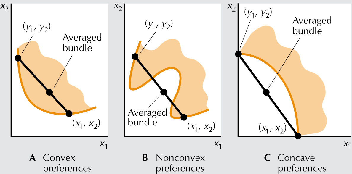
Can you think of preferences that are not convex? One possibility might be something like my preferences for ice cream and olives. I like ice cream and I like olives . . . but I don’t like to have them together! In considering my consumption in the next hour, I might be indifferent between consuming 8 ounces of ice cream and 2 ounces of olives, or 8 ounces of olives and 2 ounces of ice cream. But either one of these bundles would be better than consuming 5 ounces of each! These are the kind of preferences depicted in panel C of Figure 3.10.

Why do we want to assume that well-behaved preferences are convex? Because, for the most part, goods are consumed together. The kinds of preferences depicted in Figure 3.10, panels B and C imply that the consumer would prefer to specialize, at least to some degree, by consuming more of one good than of the other. However, the normal case is where the consumer would want to trade some of one good for the other and end up consuming some of each, rather than specializing in consuming only one of the two goods.

In fact, if we look at my preferences for monthly consumption of ice cream and olives, rather than at my immediate consumption, they would tend to look much more like Figure 3.10, panel A than panel C. Each month I would prefer having some ice cream and some olives—albeit at different times—to specializing in consuming either one for the entire month.

Finally, one extension of the assumption of convexity is the assumption of strict convexity. This means that the weighted average of two indifferent bundles is strictly preferred to the two extreme bundles. Convex preferences may have flat spots, while strictly convex preferences must have indifference curves that are “rounded.” The preferences for two goods that are perfect substitutes are convex, but not strictly convex.