Let’s consider the market for salmon again. This example meets the conditions for a competitive market because the salmon sold by one vendor is essentially the same as the salmon sold by another, and there are many individual buyers.
In Figure 3.9, we see that when the price of salmon fillets is $10 per pound, consumers demand 500 pounds and producers supply 500 pounds. This situation is represented graphically at point E, known as the point of equilibrium, where the demand curve and the supply curve intersect. At this point, the two opposing forces of supply and demand are perfectly balanced.
Notice that at $10 per pound, the quantity demanded equals the quantity supplied. At this price, and only this price, the entire supply of salmon in the market is sold. Moreover, every buyer who wants salmon is able to find some and every producer is able to sell his or her entire stock. We say that $10 is the equilibrium price because the quantity supplied equals the quantity demanded. The equilibrium price is also called the market-clearing price, because this is the only price at which no surplus or shortage of the good exists. Similarly, there is also an equilibrium quantity at which the quantity supplied equals the quantity demanded (in this example, 500 pounds). When the market is in equilibrium, we sometimes say that the market clears or that the price clears the market.
The equilibrium point has a special place in economics because movements away from that point throw the market out of balance. The equilibrium process is so powerful that it is often referred to as the law of supply and demand, the idea that market prices adjust to bring the quantity supplied and the quantity demanded into balance.
SHORTAGES AND SURPLUSES
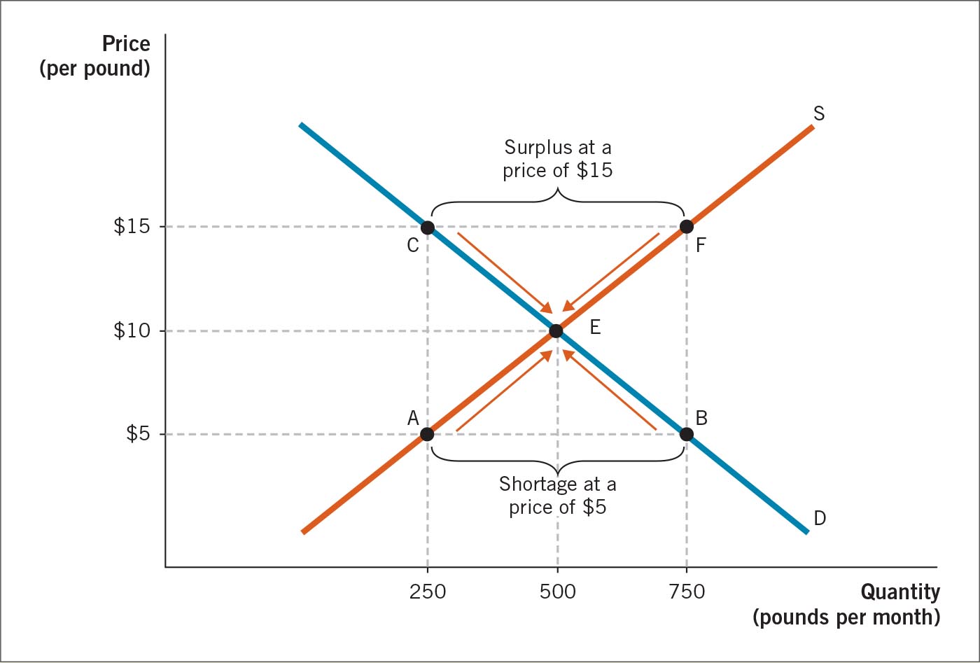
How does the market respond when it is not in equilibrium? Let’s look at two other prices for salmon shown on the y axis in Figure 3.9: $5 per pound and $15 per pound.
At a price of $5 per pound, salmon is quite attractive to buyers but not very profitable to sellers. The quantity demanded is 750 pounds, represented by point B on the demand curve (D). However, the quantity supplied, which is represented by point A on the supply curve (S), is only 250 pounds. So at $5 per pound there is an excess quantity of 750 − 250 = 500 pounds demanded. This excess demand creates disequilibrium in the market.
When there is more demand for a product than sellers are willing or able to supply, we say there is a shortage. A shortage, or excess demand, occurs whenever the quantity supplied is less than the quantity demanded. In our case, at a price of $5 per pound of salmon, there are three buyers for each pound. New shipments of salmon fly out the door, providing a strong signal for sellers to raise the price. As the market price increases in response to the shortage, sellers continue to increase the quantity they offer. You can see the increase in quantity supplied on the graph in Figure 3.9 by following the upward-sloping arrow from point A to point E. At the same time, as the price rises, buyers demand an increasingly smaller quantity, represented by the arrow from point B to point E along the demand curve. Eventually, when the price reaches $10 per pound, the quantity supplied and the quantity demanded are equal. The market is in equilibrium.
What happens when the price is set above the equilibrium point—say, at $15 per pound? At this price, salmon is quite profitable for sellers but not very attractive to buyers. The quantity demanded, represented by point C on the demand curve, is 250 pounds. However, the quantity supplied, represented by point F on the supply curve, is 750 pounds. In other words, sellers provide 500 pounds more than buyers wish to purchase. This excess supply creates disequilibrium in the market. Any buyer who is willing to pay $15 for a pound of salmon can find some because there are 3 pounds available for every customer. A surplus, or excess supply, occurs whenever the quantity supplied is greater than the quantity demanded.
When there is a surplus, sellers realize that salmon has been oversupplied, giving them a strong signal to lower the price. As the market price decreases in response to the surplus, more buyers enter the market and purchase salmon. Figure 3.9 represents this situation on the demand side by the downward-sloping arrow moving from point C to point E along the demand curve. At the same time, sellers reduce output, represented by the arrow moving from point F to point E on the supply curve. As long as the surplus persists, the price will continue to fall. Eventually, the price reaches $10 per pound. At this point, the quantity supplied and the quantity demanded are equal and the market is in equilibrium again.
In competitive markets, surpluses and shortages are resolved through the process of price adjustment. Buyers who are unable to find enough salmon at $5 per pound compete to find the available stocks; this competition drives the price up. Likewise, businesses that cannot sell their product at $15 per pound must lower their prices to reduce inventories; this desire to sell all inventory drives the price down.
Every seller and buyer has a vital role to play in the market. Venues like the Pike Place Market bring buyers and sellers together. Amazingly, market equilibrium occurs without the need for government planning to ensure an adequate supply of the goods consumers want or need. You might think that a decentralized system would create chaos, but nothing could be further from the truth. Markets work because buyers and sellers can rapidly adjust to changes in prices. These adjustments bring balance. When markets were suppressed in communist countries during the twentieth century, shortages were commonplace, in part because there was no market price system to signal that additional production was needed.
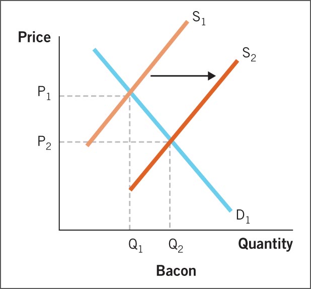
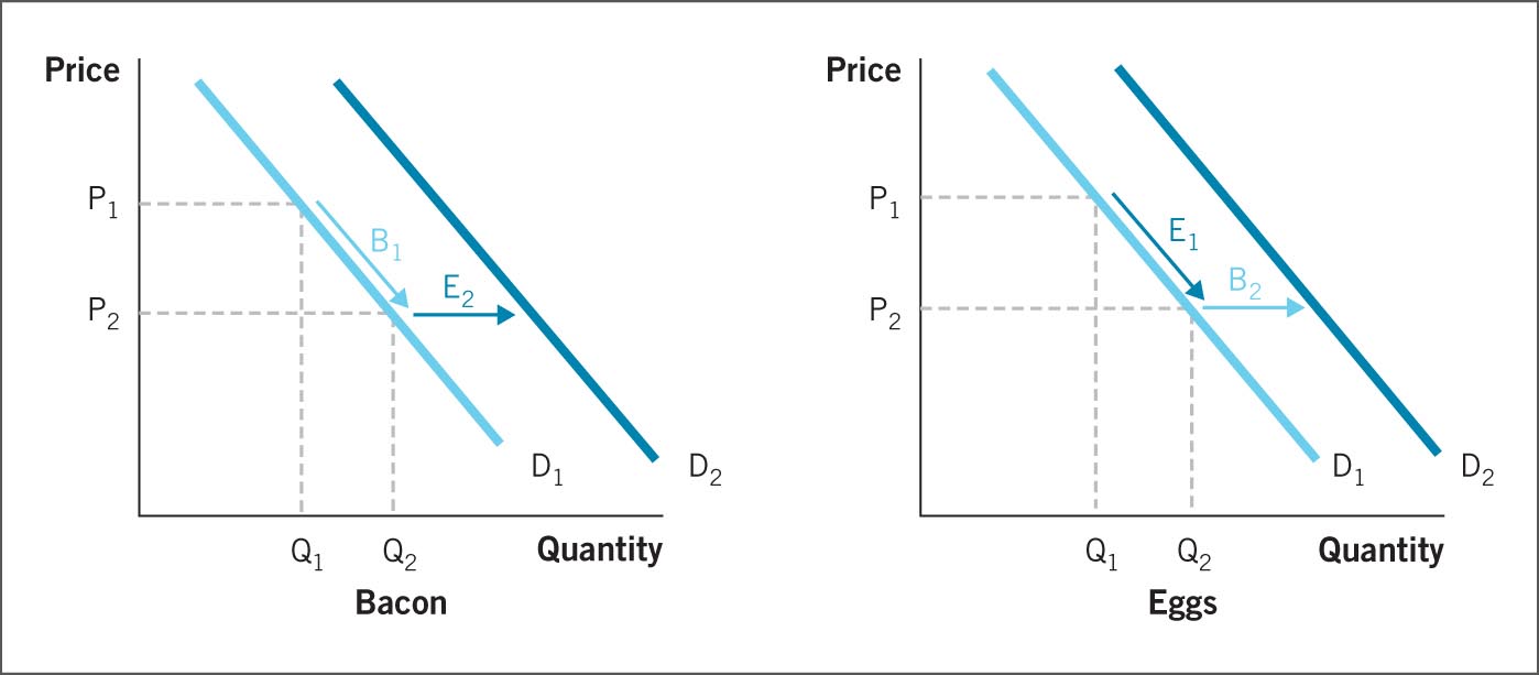
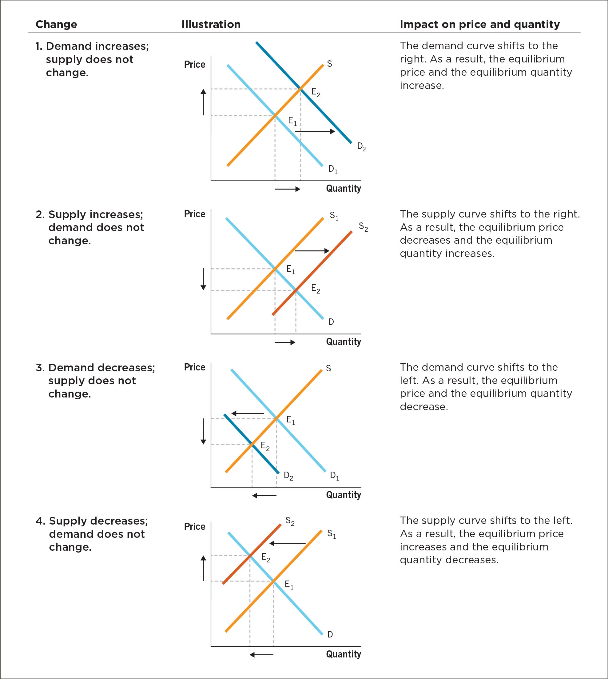
In summary, Figure 3.10 provides four examples of what happens when either the supply curve or the demand curve shifts. As you study these examples, you should develop a sense for how price and quantity are affected by changes in supply and demand. When one curve shifts, we can make a definitive statement about how price and quantity will change.
In Appendix 3A, we consider what happens when supply and demand change at the same time. There you will discover the challenges in simultaneously determining price and quantity when more than one variable changes.
 ANSWER
 ANSWER: