Even though we have learned a great deal about demand, our understanding of markets is incomplete without also analyzing supply. Let’s go back to Seattle’s Pike Place Market and focus on the behavior of producers selling goods there.
We have seen that with demand, price and output are negatively related. That is, they move in opposite directions. With supply, however, the price level and quantity supplied are positively related. That is, they move in the same direction. For instance, few producers would sell salmon if the market price were $2.50 per pound, but many would sell it at a price of $20.00 per pound. (At $20.00, producers earn more profit than they do at a price of $2.50.) The quantity supplied is the amount of a good or service that producers are willing and able to sell at the current price. Higher prices cause the quantity supplied to increase. Conversely, lower prices cause the quantity supplied to decrease.
When price increases, producers often respond by offering more for sale. As price goes down, quantity supplied also goes down. This direct positive relationship between price and quantity supplied is the law of supply. The law of supply states that, all other things being equal, the quantity supplied increases when the price rises, and the quantity supplied falls when the price falls. This law holds true over a wide range of goods and settings.
The Supply Curve
A supply schedule is a table that shows the relationship between the price of a good and the quantity supplied. The supply schedule for salmon in Table 3.2 shows how many pounds of salmon Sol Amon, owner of Pure Food Fish, would sell each month at different prices. (Pure Food Fish is a fish stand that sells all kinds of freshly caught seafood.) When the market price is $20.00 per pound, Sol is willing to sell 800 pounds. At $12.50, Sol’s quantity offered is 500 pounds. If the price falls to $10.00, he offers 400 pounds. Every time the price falls, Sol offers less salmon. This means he is constantly adjusting the amount he offers. As the price of salmon falls, so does Sol’s profit from selling it. Because Sol’s livelihood depends on selling seafood, he has to find a way to compensate for the lost income. So he might offer more cod instead.
TABLE 3.2
Pure Food Fish’s Supply Schedule for Salmon
Price of salmon (per pound)
Pounds of salmon supplied (per month)
$20.00
800
17.50
700
15.00
600
12.50
500
10.00
400
7.50
300
5.00
200
2.50
100
0.00
0
FIGURE 3.5
Pure Food Fish’s Supply Curve for Salmon
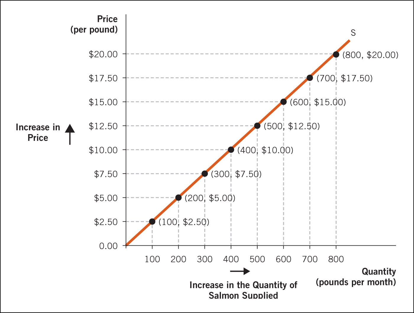
Pure Food Fish’s supply curve for salmon plots the data from Table 3.2. When the price of salmon is $10.00 per pound, Pure Food Fish supplies 400 pounds. If the price rises to $12.50 per pound, Pure Food Fish increases its quantity supplied to 500 pounds. The figure illustrates the law of supply by showing a positive relationship between price and the quantity supplied.
More information
A supply curve. On the Y-axis is price per pound of salmon and on the X-axis is quantity in pounds per month. A single linearly increasing line is the supply curve and is labeled S. There are 8 points on the line, and at each point a dashed vertical and horizontal line extend to the left and downward from the line to their respective X-axis and Y-axis points. An arrow goes up on the Y-axis and reads increase in price; an arrow on the X-axis goes right and reads Increases in the quantity of salmon shipped.
Sol and the other seafood vendors must respond to price changes by adjusting what they offer for sale in the market. This is why Sol offers more salmon when the price rises and less salmon when the price declines.
Incentives
When we plot the supply schedule in Table 3.2, we get the supply curve shown in Figure 3.5. A supply curve is a graph of the relationship between the prices in the supply schedule and the quantity supplied at those prices. As you can see in Figure 3.5, this relationship produces an upward-sloping curve. Sellers are more willing to supply the market when prices are high, because this higher price generates more profits for the business. The upward-sloping curve means that the slope of the supply curve is positive, which illustrates a direct (positive) relationship between the price and the quantity offered for sale. For instance, when the price of salmon increases from $10.00 per pound to $12.50 per pound, Pure Food Fish will increase the quantity it supplies to the market from 400 pounds to 500 pounds.
Market Supply
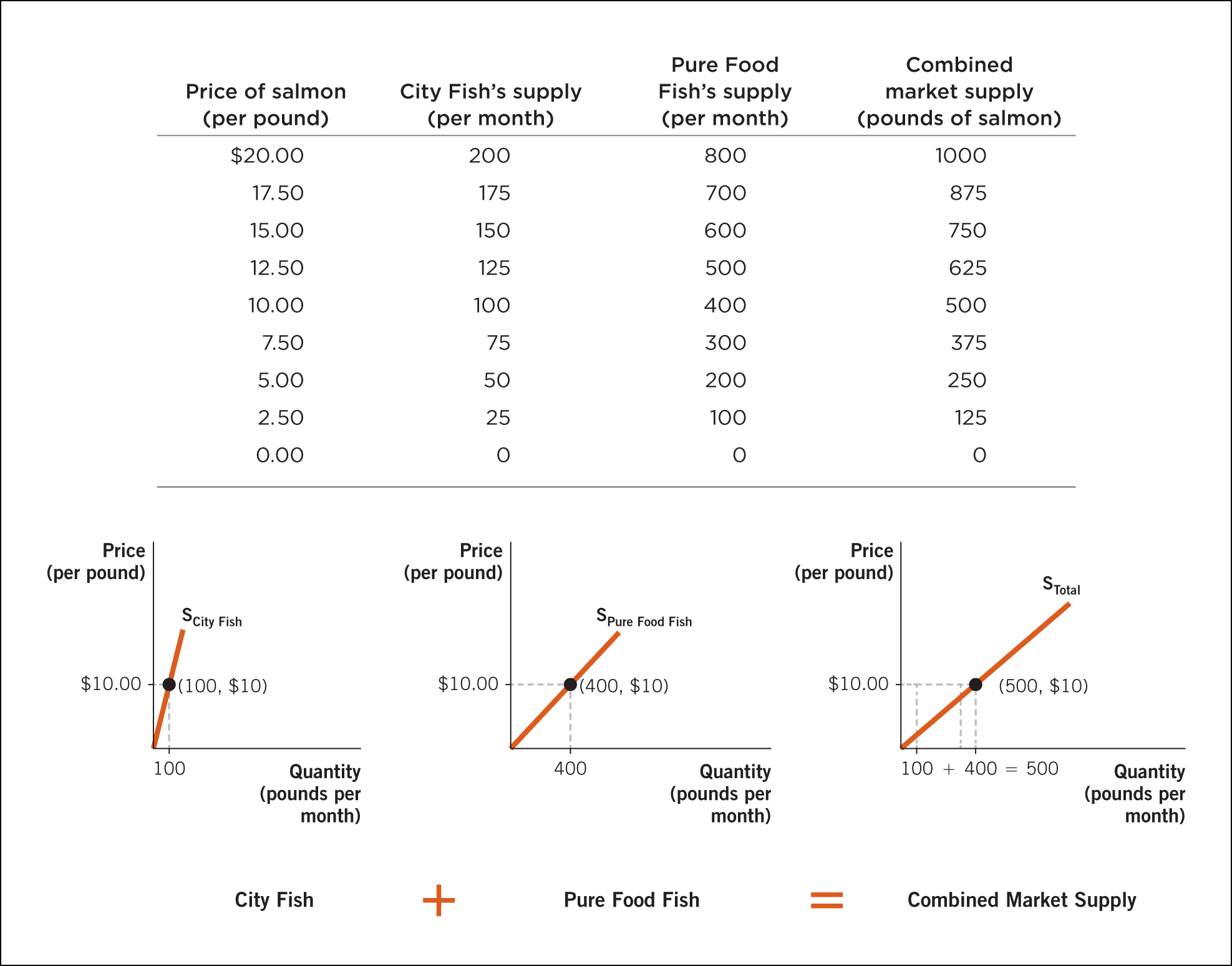
Sol Amon is not the only vendor selling fish at the Pike Place Market. The market supply is the sum of the quantities supplied by each seller in the market at each price. However, to make our analysis simpler, let’s assume that our market consists of just two sellers, City Fish and Pure Food Fish, each of which sells salmon. Figure 3.6 shows supply schedules for those two fish sellers and the combined, total-market supply schedule and the corresponding graphs.
FIGURE 3.6
Calculating Market Supply
Market supply is calculated by adding together the quantity supplied by individual vendors. The total quantity supplied, shown in the last column of the table, is illustrated in the market supply graph below.
More information
A two-part figure. At the top of the figure is a table for calculating the market supply, and below it is a graphical representation of calculating the combined market supply and a series of three supply curves. Each graph has price (per pound) on the Y-axis and quantity (pounds per month) on the X-axis and includes two vertical and horizontal dashed lines that extend outwards from a point on the graph to the respective points on the X and Y axes. The first graph is the supply curve for City fish where the supply curve is steep and goes through the point of quantity of 100 pounds and a price of 10 dollars. The next graph is the supply curve for Pure food fish where the curve is not as steep and goes through the point of a quantity of 400 and a price of 10 dollars. The final graph is the combined market supply graph which goes through the point of a quantity of 500 and a price of 10 dollars. The formula is City Fish plus Pure Food Fish equals Combined Market Supply: 100 plus 400 equals 500.
Looking at the supply schedule (the table within the figure), you can see that at a price of $10.00 per pound, City Fish supplies 100 pounds of salmon, while Pure Food Fish supplies 400 pounds. To determine the total market supply, we add City Fish’s 100 pounds to Pure Food Fish’s 400 pounds for a total market supply of 500 pounds.
Shifts of the Supply Curve
More information
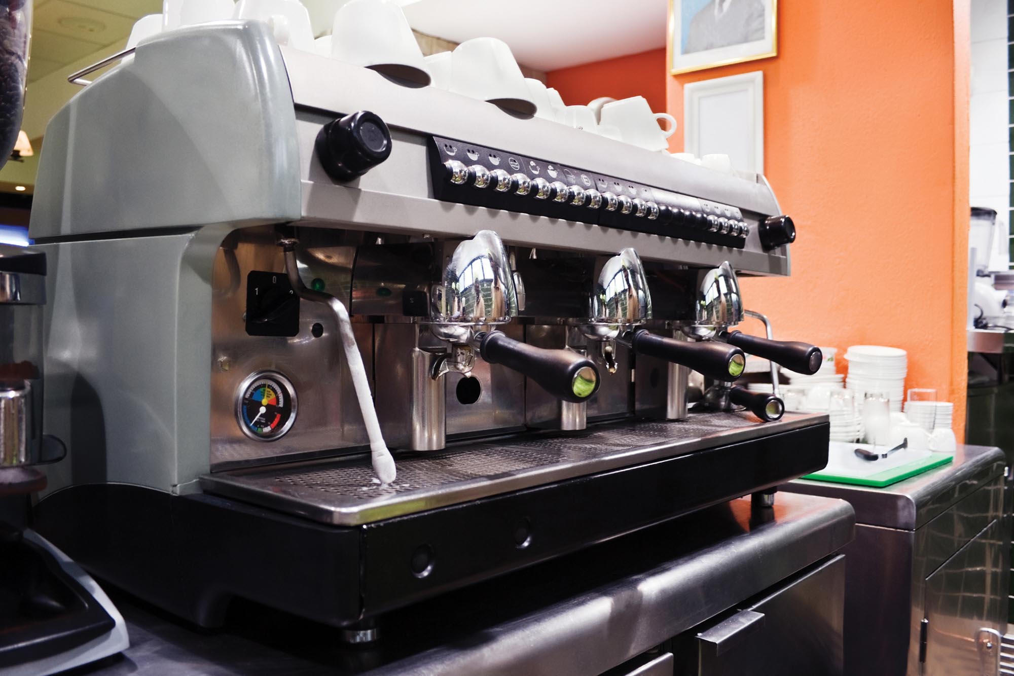
An espresso machine on a counter with one milk steamer and 3 ports to make espresso.
The first Starbucks opened in 1971 in Pike Place Market.
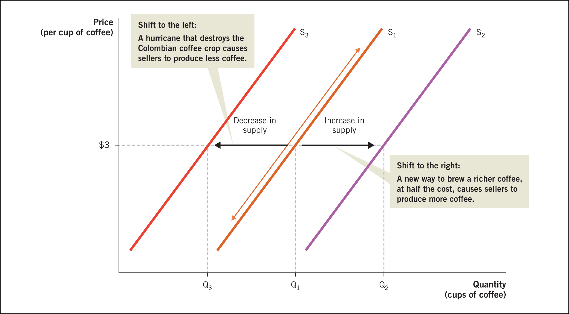
When a variable other than the price changes, the entire supply curve shifts. For instance, suppose that beverage scientists at Starbucks discover a new way to brew a richer coffee at half the cost. The new process would increase the company’s profits because its costs of supplying a cup of coffee would go down. The increased profits as a result of lower costs motivate Starbucks to sell more coffee and open new stores. Therefore, overall supply increases. Looking at Figure 3.7, we see that the supply curve shifts to the right of the original curve, from S1 to S2. Note that the retail price of coffee ($3 per cup) has not changed. When we shift the curve, we assume that price is constant and that something else has changed.
Incentives
We have just seen that an increase in supply shifts the supply curve to the right. But what happens when a variable causes supply to decrease? Suppose that a hurricane devastates the coffee crop in Colombia and reduces the world coffee supply by 10% for that year. There is no way to make up for the destroyed coffee crop, and for the rest of the year at least, the quantity of coffee supplied will be less than the previous year. This decrease in supply shifts the supply curve in Figure 3.7 to the left, from S1 to S3.
FIGURE 3.7
A Shift of the Supply Curve
When the price changes, the quantity supplied changes along the existing supply curve, illustrated here by the orange arrow. A shift in supply occurs when something other than price changes, illustrated by the black arrows.
More information
A supply curve shift. On the Y-axis is price per cup of coffee, and on the X-axis is quantity of cups of coffee. There are 3 different supply curves. The first supply curve, S1, is in the middle and goes through the point of Q1 and 3 dollars. An increase in supply from S1 causes a shift to the right to S2. Upper S subscript 2 goes through the point of Q2 and a price of 3 dollars. A decrease in supply from S1 causes a shift to the left to S3. Upper S subscript 3 goes through the point of Q3 and a price of 3 dollars.
Many variables can shift supply, but Figure 3.7 also reminds us of what does not cause a shift in supply: the price. Recall that price is the variable that causes the supply curve to slope upward. The orange arrow alongside S1 indicates that the quantity supplied will rise or fall in response to a price change. A price change causes a movement along the supply curve, not a shift in the curve.
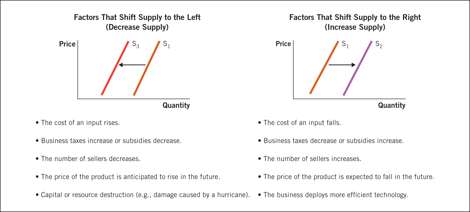
Factors that shift the supply curve include the cost of inputs, changes in technology or the production process, taxes and subsidies, the number of firms in the industry, and price expectations. Figure 3.8 provides an overview of these variables that shift the supply curve. The easiest way to keep them straight is to ask yourself a simple question: Would the change cause a business to produce more of the good or less of the good? If the change would reduce the amount of a good or service a business is willing and able to supply at every given price, the supply curve shifts to the left. If the change would increase the amount of a good or service a business is willing and able to supply at every given price, the supply curve shifts to the right.
Shifts vs. Movements Along the Supply Curve
THE COST OF INPUTS
Inputs are resources used in the production process. Inputs may include workers, equipment, raw materials, buildings, and capital goods. Each of these resources is critical to the production process. When the cost of inputs changes, so does the seller’s profit. If the cost of inputs declines, profits improve. Improved profits make the firm more willing to supply the good. So, for example, if Starbucks is able to purchase coffee beans at a significantly reduced price, it will want to supply more coffee. Conversely, higher input costs reduce profits. For instance, at Starbucks, the salaries of Starbucks store employees (or baristas, as they are commonly called) are a large part of the production cost. An increase in the minimum wage would require Starbucks to pay its workers more. This higher minimum wage would raise the cost of making coffee and make Starbucks less willing to supply the same amount of coffee at the same price.
FIGURE 3.8
Factors That Shift the Supply Curve
The supply curve shifts to the left when a factor decreases supply. The supply curve shifts to the right when a factor increases supply. (Note: A change in price does not cause a shift. Price changes cause movements along the supply curve.)
More information
Two different supply curve graphs, showing a leftward shift and a rightward shift. Both graphs include quantity on the x axis and price on the y axis, and below each supply curve is a bulleted list of factors that shift the supply curve. The first supply curve graph plots a shift of the supply curve to the left, a decrease in supply. The second supply curve graph plots a shift to the right, an increase in supply.
More information
A Starbucks employee making a coffee drink.
Baristas’ wages make up a large share of the cost of selling coffee.
CHANGES IN TECHNOLOGY OR THE PRODUCTION PROCESS
Technology encompasses knowledge that producers use to make their products. An improvement in technology enables a producer to increase output with the same resources or to produce a given level of output with fewer resources. For example, if a new espresso machine works twice as fast as the old machine, Starbucks could serve its customers more quickly, reduce long lines, and increase its sales. As a result, Starbucks would be willing to produce and sell more espressos at each price in its established menu. In other words, if the producers of a good discover a new and improved technology or a better production process, there will be an increase in supply. That is, the supply curve for the good will shift to the right.
Impact of a Shift in Supply
TAXES AND SUBSIDIES
Taxes placed on suppliers are an added cost of doing business. For example, if property taxes are increased, the cost of doing business goes up. A firm may attempt to pass along the tax to consumers through higher prices, but higher prices will discourage sales. So, in some cases, the firm will simply have to accept the taxes as an added cost of doing business. Either way, a tax makes the firm less profitable. Lower profits make the firm less willing to supply the product; thus, the supply curve shifts to the left and the overall supply declines.
The reverse is true for a subsidy. During the COVID-19 pandemic, hospitals received federal subsidies to offset the added costs associated with treating infected patients (more tests, more protective gear, more sterilizing of equipment, more laundry, and so on). In addition, airlines and small businesses received subsidies to keep workers employed while the lockdown prevented people from traveling and from going about their day-to-day business at work. As a result, more essential workers remained employed, compared to what would have happened without the subsidies.
THE NUMBER OF FIRMS IN THE INDUSTRY
We saw that an increase in total buyers (population) shifts the demand curve to the right. A similar dynamic happens with an increase in the number of sellers in an industry. Each additional firm that enters the market increases the available supply of a good. In graphic form, the supply curve shifts to the right to reflect the increased production. By the same reasoning, if the number of firms in the industry decreases, the supply curve shifts to the left.
ECONOMICS IN THE REAL WORLD
WHY DO THE PRICES OF NEW ELECTRONICS ALWAYS DROP?
The first personal computers (PCs) released in the 1980s cost as much as $10,000. Today, you can purchase a laptop computer for less than $500. When a new technology emerges, prices are initially very high and then tend to fall rapidly. The first PCs profoundly changed the way people could work with information. Before the PC, complex programming could be done only on large mainframe computers that often took up an entire room. But at first only a few people could afford a PC. What makes emerging technology so expensive when it is first introduced and so inexpensive later in its life cycle? Supply tells the story. Advances in manufacturing methods lead to an increased willingness to supply, and therefore the supply curve shifts out. When the supply expands, there is both an increase in the quantity sold and a lower price.
More information
A woman sits at her desk and types on a keyboard in front of a computer. Her desk is messy and includes open notebooks, sticky notes, a plant, and a calendar.
Why did consumers pay $5,000 for this?
Technological progress is also driving newer markets, like the market for custom shoes. 3D printing makes it possible for anyone to go online, or enter information at a kiosk in a store, and order shoes that are 100% customized. You can design the uppers, insoles, and tread however you like, and in about an hour, your shoes will be printed for you. If your two feet are slightly different sizes, you will get two different-size insoles, to match your feet perfectly. Fully customized 3D printed shoes are still pretty pricey (about $300), but the price is dropping rapidly as the process becomes more efficient and designers build templates that make it easier for customers to get exactly what they want. As the technology continues to improve, the supply curve will continue to shift out. With time, customized shoes may eventually become so cheap that almost everyone will be able to afford them easily—just like computers today!
Changes in the number of firms in a market are a regular part of business. For example, if a new pizza joint opens up nearby, more pizzas can be produced, and supply expands. Conversely, if a pizzeria closes, the number of pizzas produced falls and supply contracts.
PRICE EXPECTATIONS
A seller who expects a higher price for a product in the future may wish to delay sales until a time when the product will bring a higher price. For instance, florists know that the demand for roses spikes on Valentine’s Day and Mother’s Day. Because of higher demand, they can charge higher prices. To be able to sell more flowers during the times of peak demand, many florists work longer hours and hire temporary employees. These actions allow them to make more deliveries, so supply increases.
Likewise, the expectation of lower prices in the future will cause sellers to offer more while prices are still relatively high. This effect is particularly noticeable in the electronics sector, where newer—and much better—products are constantly being developed and released. Sellers know that their current offerings will soon be replaced by something better and that consumer demand for the existing technology will then plummet. This means that prices typically fall when a product has been on the market for a time. Because producers know that the price will fall, they supply as many of the current models as possible before the next wave of innovation cuts the price they can charge.
PRACTICE WHAT YOU KNOW
Ice Cream: Supply and Demand
More information
A little girl is sitting down and eating an ice-cream cone. A small puppy is sitting next to her and licking the ice-cream cone as well.
I scream, you scream, we all scream for ice cream.
QUESTION: Which one of the following will increase the demand for ice cream?
a decrease in the price of the butterfat used to make ice cream
a decrease in the price of ice cream
an increase in the price of the milk used to make ice cream
an increase in the price of frozen yogurt, a substitute for ice cream
AnswerAnswer:If you answered b, you made a common mistake. A change in the price of a good cannot change overall market demand; it can only cause a movement along an existing curve. So, as important as price changes are, they are not the right answer. Instead, you need to look for an event that shifts the entire curve.
Choices a and c refer to the prices of butterfat and milk. Because these are the inputs of production for ice cream, a change in their prices will shift the supply curve, not the demand curve. That leaves choice d as the only possibility. Choice d is correct because the increase in the price of frozen yogurt will cause consumers to substitute away from frozen yogurt and toward ice cream. This shift in consumer behavior will result in an increase in the demand for ice cream even though its price remains the same.
QUESTION: Which one of the following will decrease the supply of chocolate ice cream?
a medical report finding that consuming chocolate prevents cancer
a decrease in the price of chocolate ice cream
an increase in the price of chocolate, an ingredient used to make chocolate ice cream
an increase in the price of whipped cream, a complementary good
AnswerAnswer:We know that b cannot be the correct answer because a change in the price of the good cannot change supply; it can only cause a movement along an existing curve. Choices a and d would both cause a change in demand without affecting the supply curve. That leaves choice c as the only possibility. Chocolate is a necessary ingredient in the production process. Whenever the price of an input rises, profits are squeezed. The result is a decrease in supply at the existing price.
The law of supply states that, all other things being equal, the quantity supplied of a good rises when the price of the good rises, and falls when the price of the good falls.


 Answer
 Answer: