APPENDIX 03A

We have considered what would happen if supply or demand changes. But life is often more complex than that. To provide a more realistic analysis, we need to examine what happens when supply and demand both shift at the same time.

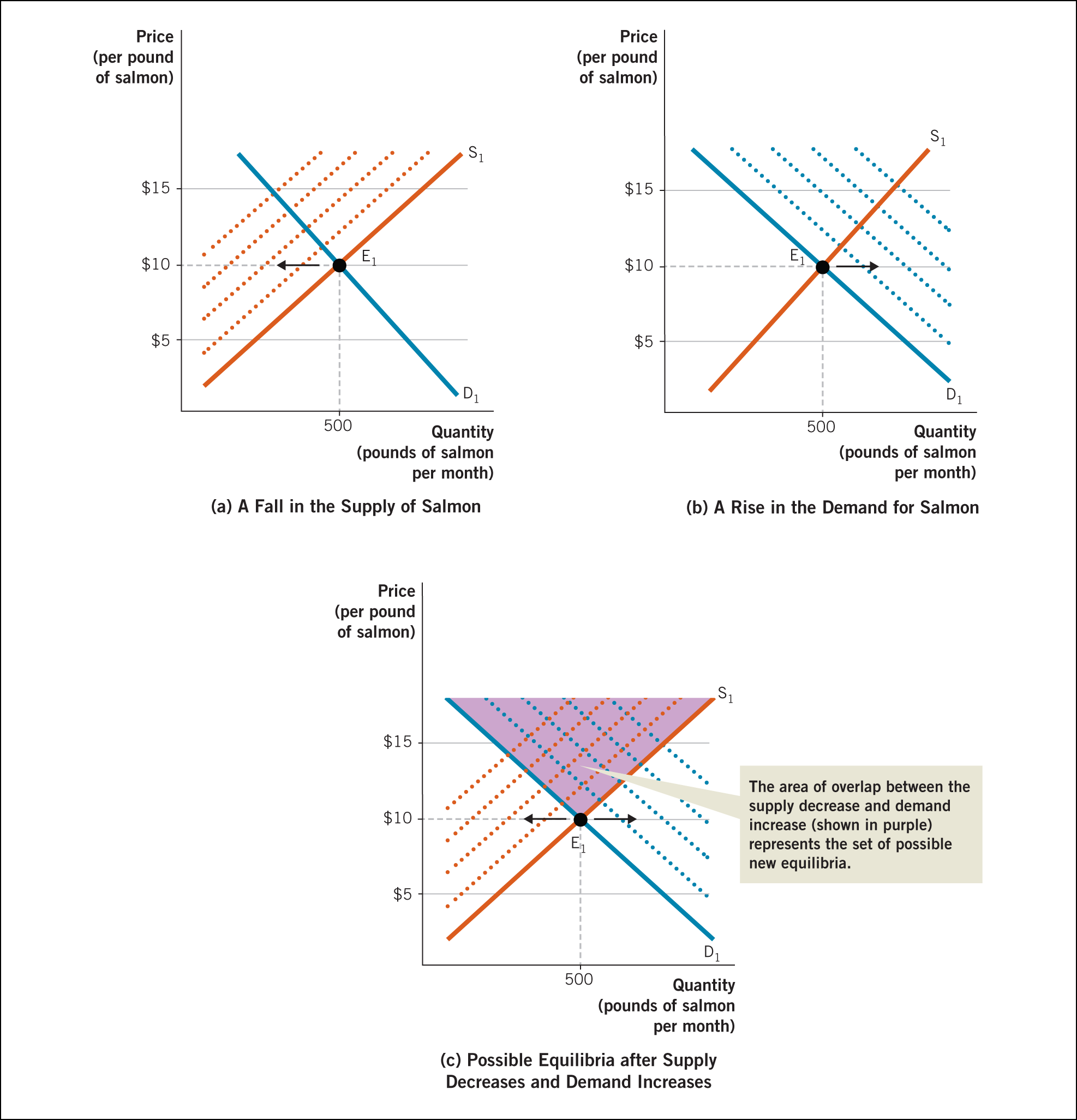
Suppose that a major drought hits the northwestern United States. The water shortage reduces both the amount of farmed salmon and the ability of wild salmon to spawn in streams and rivers. Figure 3A.1a shows the ensuing decline in the salmon supply, from S₁ progressively leftward, represented by the dotted supply curves. At the same time, a medical journal reports that people who consume at least 4 pounds of salmon a month live five years longer than those who consume an equal amount of cod. Figure 3A.1b shows the ensuing rise in the demand for salmon, from D₁ progressively rightward, represented by the dotted demand curves. This scenario leads to a twofold change. Because of the water shortage, the supply of salmon shrinks. At the same time, new information about the health benefits of eating salmon causes demand for salmon to increase.

It is impossible to predict exactly what happens to the equilibrium point when both supply and demand are shifting. We can, however, determine a region where the resulting equilibrium point must reside.

In this situation, we have a simultaneous decrease in supply and increase in demand. Since we do not know the magnitude of the supply reduction or demand increase, the overall effect on the equilibrium quantity cannot be determined. This result is evident in Figure 3A.1c, as illustrated by the purple region. The points where supply and demand cross within this area represent the set of possible new market equilibria. Because each of the possible points of intersection in the purple region occurs at a price greater than $10 per pound, we know that the price must rise. However, the left half of the purple region produces equilibrium quantities that are lower than 500 pounds of salmon, while the right half of the purple region results in equilibrium quantities that are greater than 500. Therefore, the equilibrium quantity may rise, fall, or stay the same if both shifts are of equal magnitudes.

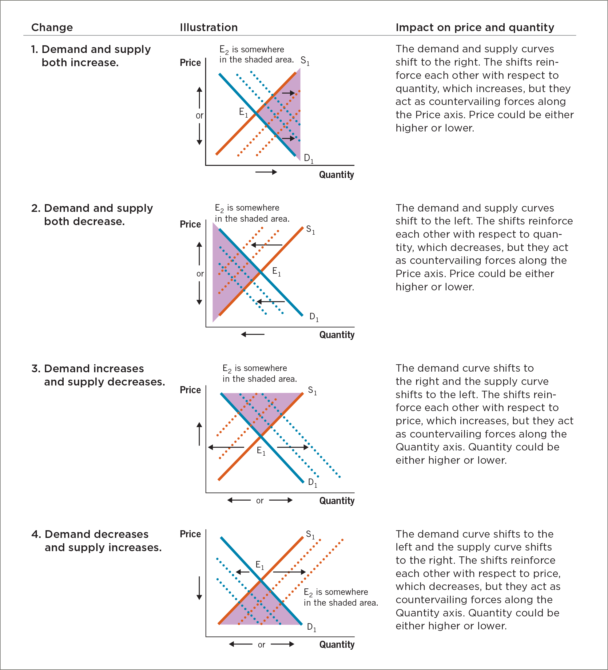
The world we live in is complex, and often more than one variable will change simultaneously. In such cases, it is not possible to be as definitive as when only one variable—supply or demand—changes. You should think of the new equilibrium not as a single point but as a range of outcomes represented by the purple area in Figure 3A.1c. Therefore, we cannot be exactly sure at what point the new price and new quantity will settle. For a closer look at four possibilities, see Figure 3A.2, where E₁ equals the original equilibrium point and the new equilibrium (E₂) lies somewhere in the purple region.

FIGURE 3A.1

A Shift in Supply and Demand

When supply and demand both shift, the resulting equilibrium can no longer be identified as an exact point. We can see this effect in (c), which combines the supply shift in (a) with the demand shift in (b). When supply decreases and demand increases, the result is that the price must rise, but the equilibrium quantity can either rise or fall, or stay the same if both shifts are of equal magnitudes.

More information

There are 3 supply-demand graphs with the title A Shift in Supply and Demand, showing the following: a fall in the supply of salmon, a rise in the demand for salmon, and possible equilibria after supply decreases and demand increases. Each graph plots price (per pound of salmon) on the Y-axis and quantity (pounds of salmon per month) on the X-axis.

FIGURE 3A.2

Price and Quantity When Demand and Supply Both Change

More information

A map shows temperatures in the Pacific Northwest during the 2021 heat wave. Much of Oregon and Washington shows triple-digit temperatures.

PRACTICE WHAT YOU KNOW

When Supply and Demand Both Change: Electric Vehicles (EVs)

QUESTION: At lunch, two friends are engaged in a heated argument. Their exchange goes like this:

The first friend begins, “The supply of EVs and the demand for EVs will both increase. I’m sure of it. I’m also sure the price of EVs will go down.”

The second friend replies, “I agree with the first part of your statement, but I’m not sure about the price. In fact, I’m pretty sure that EV prices will rise.”

They go back and forth endlessly, each unable to convince the other, so they turn to you for advice. What do you say to them?

Answer Answer: Either of your friends could be correct. In this case, supply and demand both shift out to the right, so we know that the quantity bought and sold will increase. However, an increase in supply would normally lower the price, and an increase in demand would typically raise the price. Without knowing which of these two effects on price is stronger, you can’t predict how price will change. The overall price will rise if the increase in demand is larger than the increase in supply. However, if the increase in supply is larger than the increase in demand, prices will fall. But your two friends don’t know which condition will be true—so they’re locked in an argument that neither can win. As an aside, Tesla came out with its priciest models first and is working its way down the affordability scale, which suggests that it is betting on EV prices going down over time.

More information

A smiling woman charges up her family’s S U V.

ECONOMICS IN THE REAL WORLD

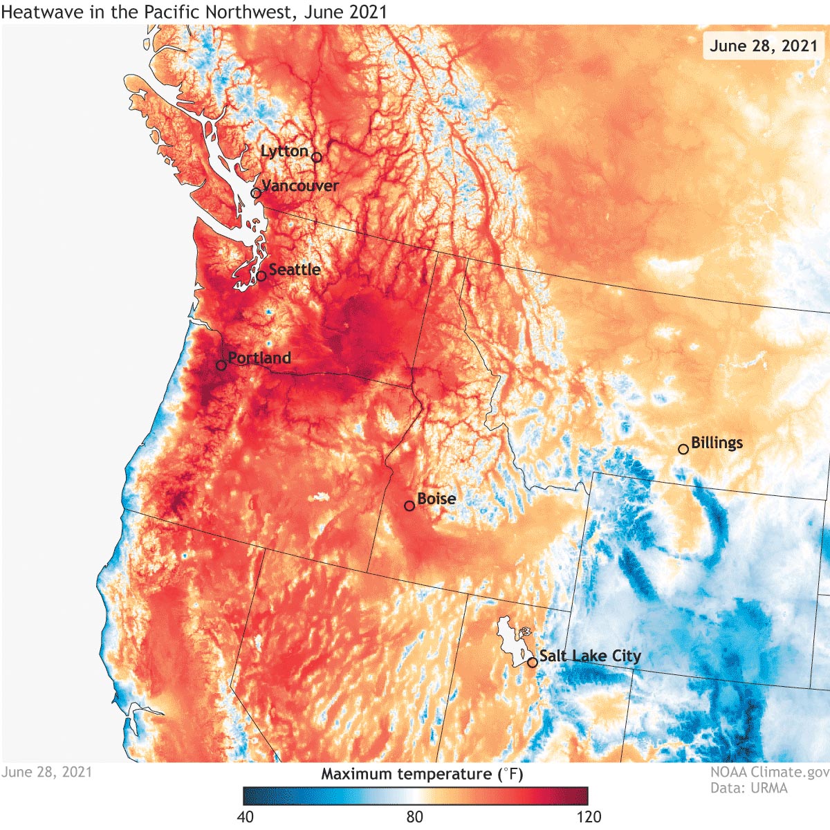
HEAT DOME ECONOMICS

In 2021, an unprecedented atmospheric heat dome brought record temperatures to the Pacific Northwest. Portland reached 116 degrees, Seattle topped out at 108, and Quillayute, Washington, on the Pacific coast, reached 110—an astonishing 45 degrees above average. But the effect was even stronger north of the border. Lytton, British Columbia, reached 121 degrees, breaking the previous temperature record for all of Canada by a whopping 8 degrees. To put this into perspective: it was hotter in Lytton than has ever been recorded in Las Vegas, 1,000 miles to the south.

The economic effects of the 2021 heat dome provide a textbook example of a positive demand shock and negative supply shock (a “shock” is an unexpected event) hitting at the same time.

First, the positive demand shock. It is easy to understand. Unprecedented heat dramatically increased (that’s why we say “positive”) the demand for electricity in the Pacific Northwest, because much more electricity than usual was needed to cool homes.

Second, the negative supply shock. It turns out that excessive heat also stresses the existing electric grid, leading to rolling blackouts, thus lowering (that’s why we say “negative”) supplies of electricity to cool homes. Just when people needed electricity the most, it was in short supply.

Third, the complication. The extreme temperatures worsened the already dry conditions throughout the Pacific Northwest. Because this area relies on hydroelectric power more than any other part of the country, the heat dome made it even harder for supply to meet peak demand in the future. As you can probably guess, “even harder” quickly translates into “even more expensive.”

More information

A table with 3 columns and 4 rows titled Price and Quantity When Demand and Supply Both Change has the following column headers: change, illustration, and impact on price and quantity. Each illustration is a graph with supply and demand curves showing equilibrium points with quantity on the x axis and price on the y axis with linear supply curves (S) with a positive slope, and linear demand curves (D) with a negative slope which intersect at equilibrium points (E).