Data gathering must follow a plan, which is the research design. No one design is suitable for all topics; according to what one wants to study, different designs may be appropriate, inappropriate, or even impossible. Research designs in psychology (and all of science) come in three basic types: case, experimental, and correlational.
Case Method
The simplest, most obvious, and most widely used way to learn about something is, as Henry Murray advised, just to look at it. According to legend, Isaac Newton was sitting under a tree when an apple hit him on the head, and that got him thinking about gravity. A scientist who keeps her eyes and ears open can find all sorts of phenomena that can stimulate new ideas and insights. The case method involves closely studying a particular event or person in order to find out as much as possible.
Whenever an airplane crashes in the United States, the National Transportation Safety Board (NTSB) sends a team and launches an intensive investigation. In January 2000, an Alaska Airlines plane went down off the California coast; after a lengthy analysis, the NTSB concluded this happened because a crucial part, the jackscrew assembly in the plane’s tail, had not been properly greased (Alonso-Zaldivar, 2002). This conclusion answered the specific question of why this particular crash happened, and it also had implications for the way other, similar planes should be maintained (i.e., don’t forget to grease the jackscrew!). At its best, the case method yields not only explanations of particular events, but also useful lessons and perhaps even scientific principles.
All sciences use the case method. When a volcano erupts, geologists rush to the scene with every instrument they can carry. When a fish previously thought long extinct is pulled from the bottom of the sea, ichthyologists stand in line for a closer look. Medicine has a tradition of “grand rounds” where doctors in training look at individual patients. Even business school classes spend long hours studying examples of companies that succeeded and failed. But the science best known for its use of the case method is psychology, and in particular personality psychology. Sigmund Freud built his famous theory from experiences with patients who offered interesting phobias, weird dreams, and traumatic memories (see Chapter 10). Psychologists who are not psychoanalytically inclined have also used cases; Gordon Allport argued for the importance of studying particular individuals in depth, and even wrote an entire book about one person (Allport, 1965).20 More recently, psychologist Dan McAdams has argued that it is important to listen to and understand “life narratives,” the unique stories individuals construct about themselves (McAdams et al., 2004).
The case method has several advantages. One is that, above all other methods, it is the one that feels like it does justice to the topic. A well-written case study can be like a short story or even a novel; in general, the best thing about a case study is that it describes the whole phenomenon and not just isolated variables.
A second advantage is that a well-chosen case study can be a source of ideas. It can illuminate why planes crash (and perhaps prevent future disasters) and reveal general facts about the inner workings of volcanoes, the body, businesses, and, of course, the human mind. Newton’s apple got him thinking about gravity in a whole new direction; nobody suspected that grease on a jackscrew could be so important; and Freud generated an astounding number of ideas just from looking closely at himself and his patients.
A third advantage of the case method is often forgotten: Sometimes, the method is absolutely necessary. A plane goes down; we must at least try to understand why. A patient appears, desperately sick; the physician cannot just say, “More research is needed,” and send her away. Psychologists, too, sometimes must deal with particular individuals, in all their wholeness and complexity, and base their efforts on the best understanding they can quickly achieve.
The big disadvantage of the case method is obvious. The degree to which its findings can be generalized is unknown. Each case contains numerous, and perhaps literally thousands, of specific facts and variables. Which of these are crucial, and which are incidental? Once a specific case has suggested an idea, the idea needs to be checked out; for that, the more formal methods of science are required: the experimental method and the correlational method.
For example, let’s say you know someone who has a big exam coming up. It is very important to him, and he studies hard. However, he freaks out while taking the test. Even though he knows the subject matter, he gets a poor grade. Have you ever seen this happen? If you have (I know I have), then this case might cause you to think of a general hypothesis: Anxiety harms test performance. That sounds reasonable, but does this one example prove the hypothesis is true? Not really, but it was the source of the idea. The next step is to find a way to do research to test this hypothesis. You could do this in either of two ways: with an experiment or a correlational study.
An Experimental and a Correlational Study
The experimental way to examine the relationship between anxiety and test performance would be to get a group of research participants and randomly divide them into two groups. It is important that they be assigned randomly because then you can presume that the two groups are more or less equal in ability, personality, and other factors. If they aren’t, then something probably wasn’t random. For example, if one group of subjects was recruited by one research assistant and the other group was recruited by another, the experiment is already in deep trouble, because the two assistants might—accidentally or on purpose—tend to recruit different kinds of participants. It is critical to ensure that nothing beyond sheer chance affects whether a participant is assigned to one condition or the other.
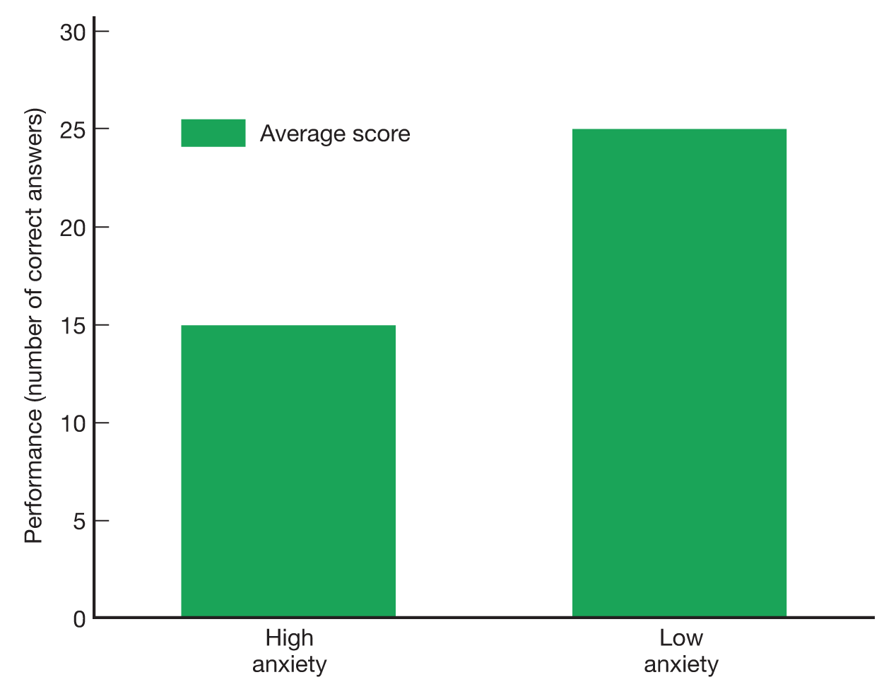
Now it’s time for the experimental procedure. Do something to one of the groups that you expect will make the members of that group anxious, such as telling them, “Your future success in life depends on your performance on this test” (but see the discussion on ethics and deception in Chapter 3). Tell the other group that the test is “just for practice.” Then give both groups something like a 30-item math test. If anxiety hurts performance, then you would expect the participants in the “life depends” group to do worse than the participants in the “practice” group. You might write the results down in a table like Table 2.3 and display them on a chart like Figure 2.4. In this example, the mean (average) score of the high-anxiety group indeed seems lower than that of the low-anxiety group. You would then do a statistical test, probably one called a t-test in this instance, to see if the difference between the means is larger than one would expect from chance variation alone.
Table 2.3PARTIAL DATA FROM A HYPOTHETICAL EXPERIMENT ON THE EFFECT OF ANXIETY ON TEST PERFORMANCE
Participants in the High-Anxiety Condition, No. of Correct Answers
Participants in the Low-Anxiety Condition, No. of Correct Answers
Sidney = 13
Ralph = 28
Jane = 17
Susan = 22
Kim = 20
Carlos = 24
Bob = 10
Thomas = 20
Patricia = 18
Brian = 19
Etc.
Etc.
Mean = 15
Mean = 25
Note: Participants were assigned randomly to either the low-anxiety or high-anxiety condition, and the average number of correct answers was computed within each group. When all the data were in, the mean for the high-anxiety group was 15 and the mean for the low-anxiety group was 25. These results would typically be plotted as in Figure 2.4.
Figure 2.4Plot of the Results of a Hypothetical Experiment Participants in the high-anxiety condition got an average of 15 out of 30 answers correct on a math test, and participants in the low-anxiety condition got an average of 25 correct.
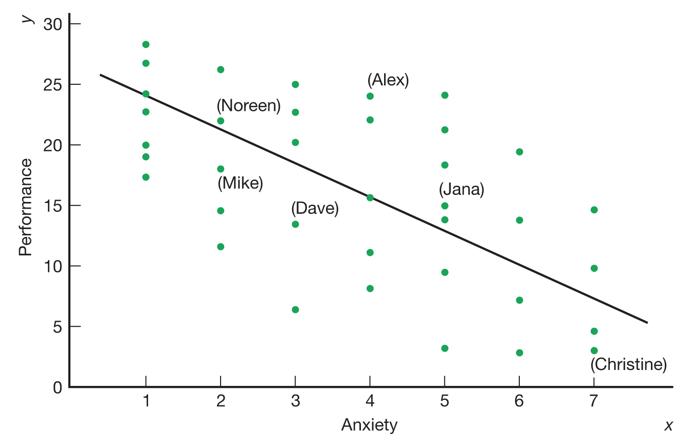
The correlational way to examine the same hypothesis would be to measure the amount of anxiety that your participants bring into the lab naturally, rather than trying to induce anxiety artificially. In this method, everybody is treated the same. There are no experimental groups. Instead, as soon as the participants arrive, you give them a questionnaire asking them to rate how anxious they feel on a scale of 1 to 7. Then you administer the math test. Now the hypothesis would be that if anxiety hurts performance, then those who scored higher on the anxiety measure will score worse on the math test than will those who scored lower on the anxiety measure. The results typically are presented in a table like Table 2.4 and then in a chart like Figure 2.5. Each of the points on the chart, which is called a scatter plot, represents an individual participant’s pair of scores, one for anxiety (plotted on the horizontal, or x-axis) and one for performance (plotted on the vertical or y-axis). If a line drawn through these points leans in a downward direction from left to right, then the two scores are negatively correlated, which means that as one score gets higher, the other gets smaller. In this case, as anxiety gets higher, performance tends to get worse, which is what you predicted. A statistic called a correlation coefficient (described in detail in Chapter 3) reflects just how strong this trend is. The statistical significance of this correlation can be checked to see whether it is large enough, given the number of participants in the study, to conclude that it would be highly unlikely if the real correlation, in the population, were zero.
Table 2.4PARTIAL DATA FOR A HYPOTHETICAL CORRELATIONAL STUDY OF THE RELATIONSHIP BETWEEN ANXIETY AND TEST PERFORMANCE
Participant
Anxiety (x)
Performance (y)
Dave
3
12
Christine
7
3
Mike
2
18
Alex
4
24
Noreen
2
22
Jana
5
15
Etc
. . .
. . .
Note: An anxiety score (denoted x) and a performance score (denoted y) are obtained from each participant. The results are then plotted in a manner similar to that shown in Figure 2.5.
Figure 2.5Plot of the Results of a Hypothetical Correlational Study Participants who had higher levels of anxiety tended to get lower scores on the math test. The data from the participants represented in Table 2.4 are included, along with others not represented in the table.
Comparing the Experimental and Correlational Methods
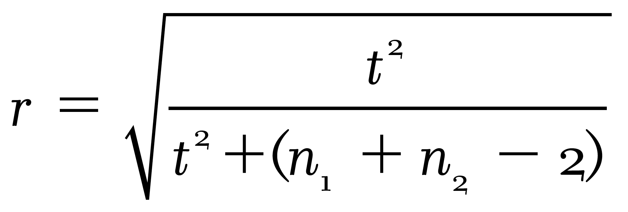
The experimental and correlational methods are often discussed as if they were utterly different. I hope this example makes clear that they are not. Both methods attempt to assess the relationship between two variables; in the example just discussed, they were “anxiety” and “test performance.” A further, more technical similarity is that the statistics used in the two studies are interchangeable—the t statistic from the experiment can be converted, using simple algebra, into a correlation coefficient (traditionally denoted by r), and vice versa. (Footnote 17 in Chapter 3 gives the exact formula.) The only real difference between the two designs is that in the experimental method, the presumably causal variable—anxiety—is manipulated, whereas in the correlational method, the same variable is measured as it already exists.
This single difference is very important. It gives the experimental method a powerful advantage: the ability to ascertain what causes what. Because the level of anxiety in the experiment was manipulated by the experimenter, and not just measured as it already existed, you know what caused it. The only possible path is anxiety ⟶ performance. In the correlational study, you can’t be so sure. Both variables might be the result of some other, unmeasured factor. For example, perhaps some participants in your correlational study were sick that day, which caused them to feel anxious and perform poorly. Instead of a causal pathway with two variables, the truth might be more like:
the truth might be more like:
For obvious reasons, this potential complication with correlational design is called the third-variable problem.
A slightly different problem arises in some correlational studies, which is that either of the two correlated variables might actually have caused the other. For example, if one finds a correlation between the number of friends one has and happiness, it might be that having friends makes one happy, or that being happy makes it easier to make friends. Or, in a diagram, the truth of the matter could be either
or
The correlation itself cannot tell us the direction of causality—indeed, it might (as in this example) run in both directions:
You may have heard the expression “Correlation is not causality.” It’s true. Correlational studies are informative, but raise the possibility that both of two correlated variables were caused by an unmeasured third variable, that either of them might have caused the other, or even that both of them cause each other. Teasing these possibilities apart is a major methodological task, and complex statistical methods such as structural equation modeling have been developed to try to help.
The experimental method is not completely free of complications either, however. One problem is that you can never be sure exactly what you have manipulated and, therefore, of where the actual causality was located. In the earlier example, it was presumed that telling participants that their future lives depend on their test scores would make them anxious. The results then confirmed the hypothesis: Anxiety hurts performance. But how do you know the statement made them anxious? Maybe it made them angry or disgusted at such an obvious lie. If so, then it could have been anger or disgust that hurt their performance. You only know what you manipulated at the visible, operational level—you know what you said to the participants. The psychological variable that you manipulated, however—the one that actually affected behavior—was invisible and can only be inferred. (This difficulty is related to the problem with interpreting B data discussed earlier in this chapter.) You might also recognize this difficulty as another version of the third-variable problem just discussed. Indeed, the third-variable problem affects both correlational and experimental designs, but in different ways.
A second complication with the experimental method is that it can create levels of a variable that are unlikely or even impossible in real life. Assuming the experimental manipulation worked as intended, which in this case seems like a big assumption, how often is your life literally hanging in the balance when you take a math test? Any extrapolation to the levels of anxiety that ordinarily exist during exams could be highly misleading. Moreover, maybe in real-life exams most people are moderately anxious. But in the experiment, two groups were artificially created: One was presumably highly anxious; the other (again, presumably) was not anxious at all. In real life, both groups may be rare. Therefore, the effect of anxiety on performance may be exaggerated. The correlational method, by contrast, assesses levels of anxiety that already exist in the participants. Thus, they are more likely to represent anxiety as it realistically occurs.
This conclusion highlights an important way in which experimental and correlational studies complement each other. An experiment can determine whether one variable can affect another, but not how often or how much it actually does, in real life. For that, correlational research is required. Also, notice how the correlational study included seven levels of anxiety (one for each point on the anxiety scale), whereas the experimental study included only two (one for each condition). Therefore, the results of the correlational study may be more precise.
A third disadvantage particular to the experimental method is that, unlike correlational studies, experiments often require deception. Correlational studies don’t. I will discuss the ethics of deception in Chapter 3.
The final disadvantage of the experimental method is the most important one. Sometimes experiments are simply not possible. For example, if you want to know the effects of child abuse on self-esteem in adulthood, all you can do is try to assess whether people who were abused as children tend to have low self-esteem, which would be a correlational study. The experimental equivalent is not possible. You cannot assemble a group of children and randomly abuse half of them. Moreover, the main thing personality psychologists usually want to know is how personality traits or other stable individual differences affect behavior. But you cannot make half of the participants extraverted and the other half introverted; you must accept the personalities that participants bring into the laboratory.
Many discussions of correlational and experimental designs, including those in many textbooks, conclude that the experimental method is obviously superior. This conclusion is wrong. Experimental and correlational designs both have advantages and disadvantages, as we have seen, and ideally a complete research program would include both.
A research technique that establishes the causal relationship between an independent variable (x) and dependent variable (y) by randomly assigning participants to experimental groups characterized by differing levels of x, and measuring the average behavior (y) that results in each group.
A research technique that establishes the relationship (not necessarily causal) between two variables, traditionally denoted x and y, by measuring both variables in a sample of participants.
A diagram that shows the relationship between two variables by displaying points on a two-dimensional plot. Usually the two variables are denoted x and y, each point represents a pair of scores, and the x variable is plotted on the horizontal axis while the y variable is plotted on the vertical axis.
A number between –1 and +1 that reflects the degree to which one variable, traditionally called y, is a linear function of another, traditionally called x. A negative correlation means that as x goes up, y goes down; a positive correlation means that as x goes up, so does y; a zero correlation means that x and y are unrelated.
Notes
20. The identity of this person was supposed to be secret. Years later, historians established it was Allport’s college roommate’s mother.