2.5 Fluorescence Microscopy, FISH, and Chemical Imaging Microscopy
Fluorescence microscopy (also called epifluorescence microscopy) is a powerful tool for identifying specific kinds of microbes, such as pathogens or members of environmental communities. Fluorescence also reveals specific cell parts at work, such as division proteins in the act of accomplishing cell fission. The profound importance of fluorescence for microbial discovery was acknowledged by the awarding of the 2008 Nobel Prize in Chemistry to Osamu Shimomura, Martin Chalfie, and Roger Tsien for the discovery and development of green fluorescent protein (GFP). Fluorescence microscopy can now be coupled to new tools of chemical imaging, which reveals the actual chemistry of cell parts under microscopy.
What Is Fluorescence?
In fluorescence microscopy, the specimen absorbs light of a defined wavelength and then emits light of lower energy, hence longer wavelength; thus, the specimen is said to “fluoresce.” Some microbes, such as cyanobacteria and algae, fluoresce on their own (autofluorescence), owing to endogenous fluorescent molecules such as chlorophyll. Chlorophyll autofluorescence has important applications in environmental monitoring of algae and cyanobacteria.
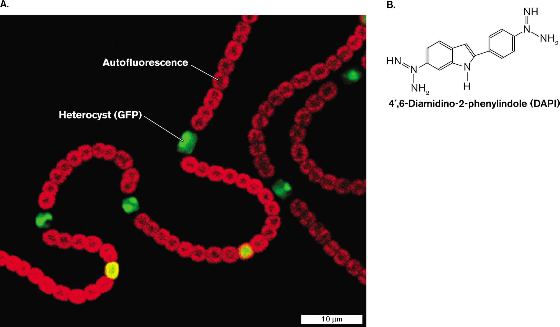
For other aims, specific parts of the cell are labeled with a fluorophore, a fluorescent dye or protein. In Figure 2.26A, cells of the cyanobacterium Nostoc sp. PCC 7120 (formerly Anabaena sp. PCC 7120) show autofluorescence (red) arising from their chlorophyll. Every tenth cell or so, however, develops as a nitrogen-fixing heterocyst that lacks chlorophyll. In the sample shown, the bacteria are engineered such that heterocysts express a nitrogen-stress gene fused to a gene that encodes GFP. (We’ll discuss this technique shortly.) Thus, the two different colors of fluorescence distinguish between the cyanobacterial cells conducting photosynthesis and the heterocysts conducting nitrogen fixation.
Fluorescence microscopy is also used by marine ecologists to reveal tiny bacteria and plankton growing in seawater, a highly dilute natural environment (discussed in Chapter 21). Such observations support the study of microbial responses to climate change. Microbes, including viruses, bacteria, and protists, are detected by fluorescence of DNA-specific stains such as DAPI (4′, 6-diamidino-2-phenylindole; Fig. 2.26B). The advantage of DAPI fluorescent stain is that it detects only cells whose DNA is intact, distinguishing them from environmental debris.
More information
An image taken with a fluorescent microscope and the molecular structure of D A P I are shown.
An image of autofluorescence and fluorescence in Cyanobacteria. Long chains of cocci are shown, with each coccus about 1 micrometer in diameter. Most of the cocci express autofluorescence and appear red. A few cocci are heterocysts expressing a nitrogen stress gene fused to G F P, these appear green.
The molecular structure of 4 prime, 6-Diamidino-2-phenylindole, or D A P I. This consists of benzene bonded to a 4-membered carbon ring at the right. C 5 of the benzene is single bonded to nitrogen, and nitrogen is single bonded to ammonia and double-bonded to H N. C 3 of the 4-membered carbon ring is substituted by nitrogen single bonded to hydrogen. C 2 of the 4-membered carbon ring is single bonded to another benzene ring at the top, in which C 2 is single bonded to nitrogen, and nitrogen is single bonded to ammonia and double-bonded to N H.
FIGURE 2.26 ■Fluorescence microscopy.A. Cyanobacteria show chlorophyll-based autofluorescence (red) and fluorescence from heterocysts (green) expressing a nitrogen-stress gene fused to GFP. B. The molecule DAPI is used as a fluorescent stain that specifically labels DNA. ALICIA M. MURO-PASTOR
Excitation and Emission
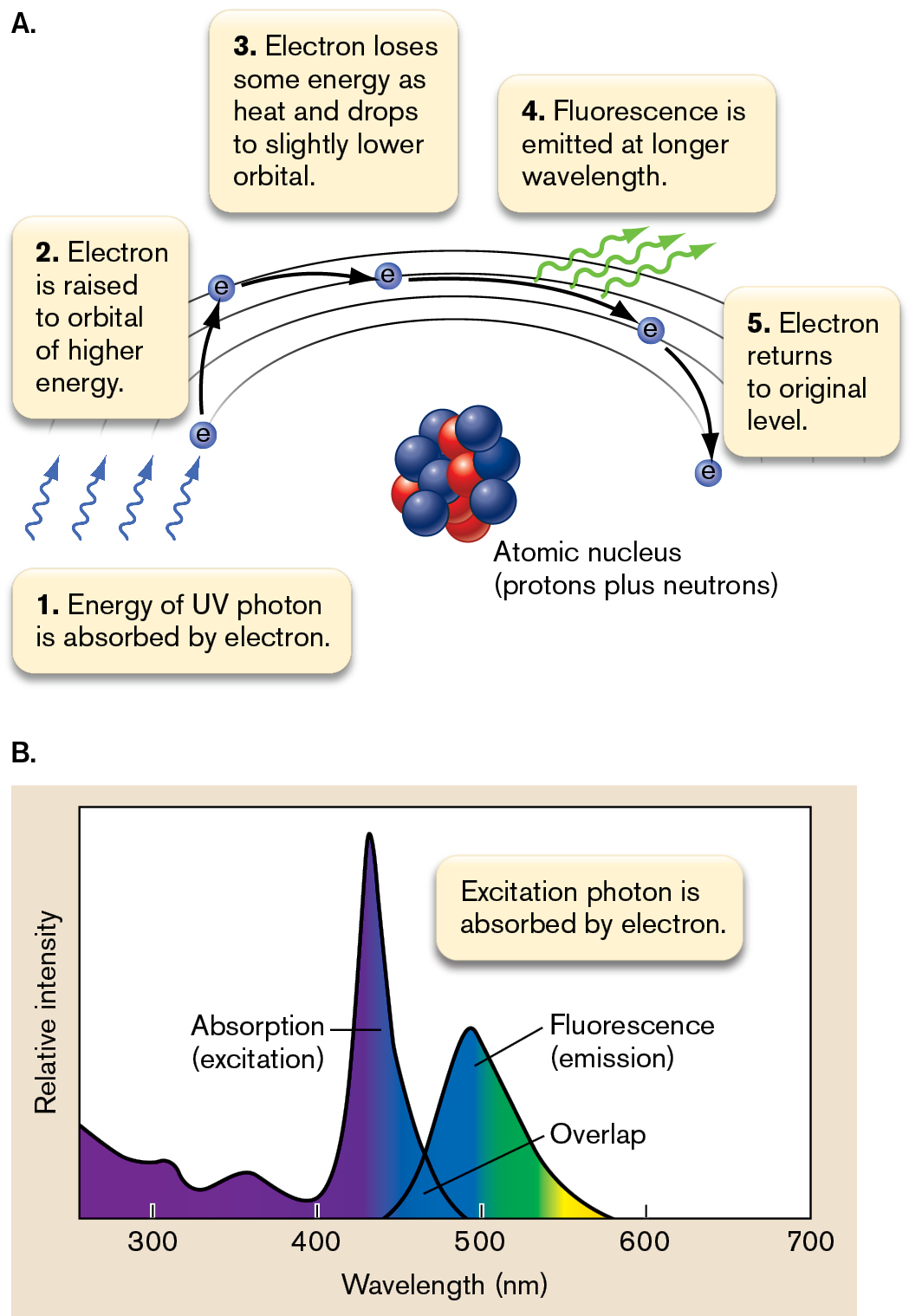
How and when does a molecule fluoresce? Fluorescence occurs when a molecule absorbs light of a specific wavelength (the excitation wavelength) that has just the right energy needed to raise an electron to a higher-energy orbital (Fig. 2.27). Because this higher-energy electron state is unstable, the electron decays to an orbital of slightly lower energy, while losing some energy as heat. The electron then falls to its original level by emitting a photon of less energy and longer wavelength (the emission wavelength). The emitted photon has a longer wavelength (less energy) because part of the electron’s energy of absorption was lost as heat.
More information
An illustration and a graph describe the concept of fluorescence.
An illustration shows the concept of fluorescence at the molecular level. A model of an atomic nucleus is comprised of protons and neutrons. The steps involved are as follows: Step 1: Energy of the U V photon is absorbed by the electron. Step 2: The electron is raised to an orbital of higher energy. Step 3: Electron loses some energy as heat and drops to a slightly lower orbital. Step 4: Fluorescence is emitted at a longer wavelength. Step 5: Electron returns to its original level.
A graph shows two peaks for absorption and fluorescence. The x-axis represents wavelength in nanometers ranging from 300 to 700 in increments of 100. The y-axis represents relative intensity without units. The first peak is labeled Absorption, or excitation. This peak starts below the midpoint of the y-axis at 400 nanometers in wavelength, then rises to a tall peak at 450 nanometers, and to a relative intensity of 0 at 500 nanometers. The second is labeled fluorescence, or emission. This peak starts at a wavelength of 450 nanometers, rises to a small peak at 500 nanometers, and drops to 0 relative intensity at 598 nanometers. The two curves intersect at 475 nanometers, the area between is labeled as overlap. The corresponding text reads excitation photon is absorbed by the electron.
FIGURE 2.27 ■Fluorescence. Energy gained from UV absorption is released as heat and as a photon of longer wavelength in the visible region. A. Fluorescence on the molecular level. B. Comparison of absorption and emission spectra for a fluorophore.
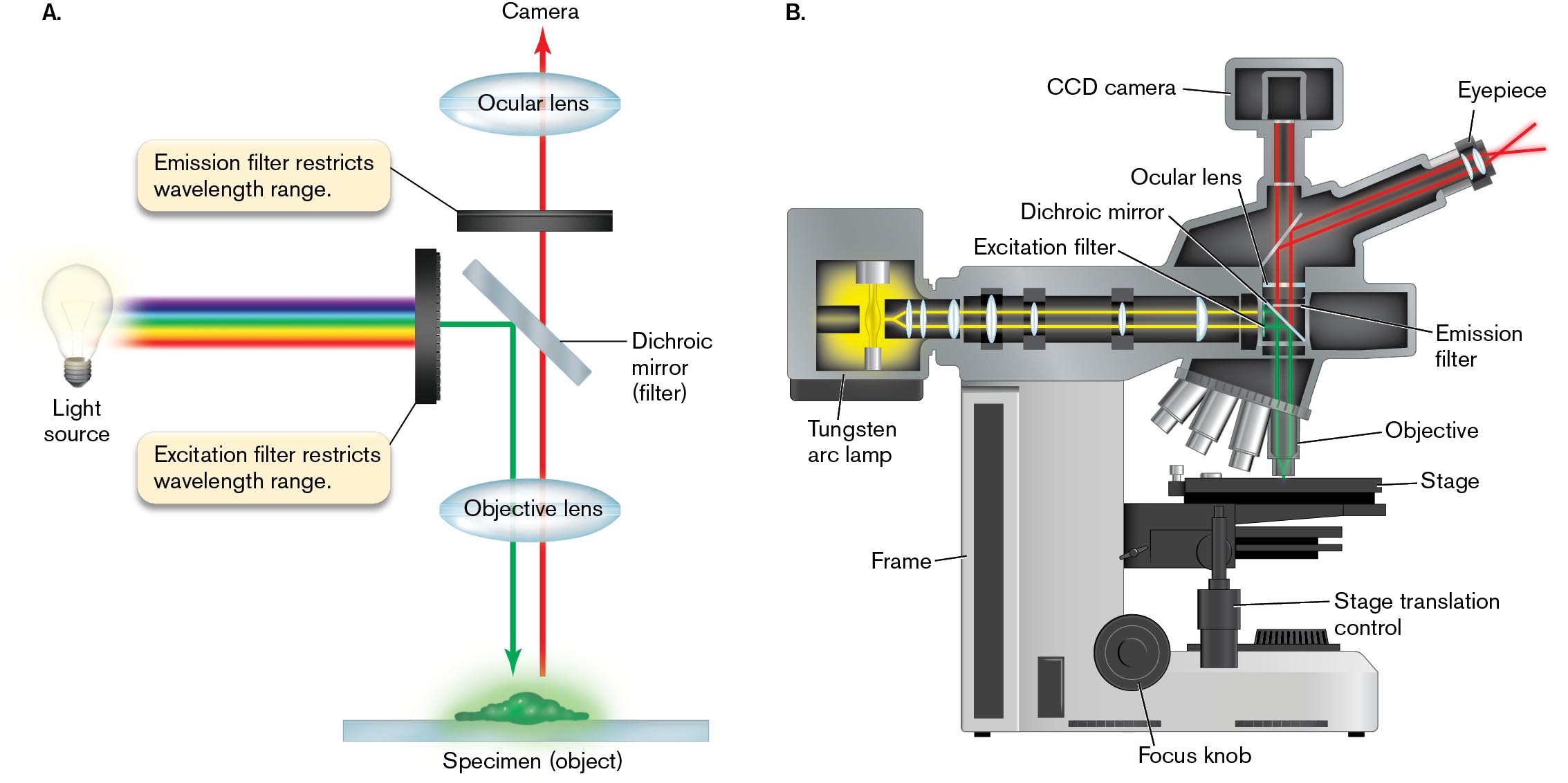
The optical system for fluorescence microscopy uses filters to limit the source light to the wavelength range of excitation and the specimen’s emitted light to the wavelength range of emission (Fig. 2.28). The wavelengths of excitation and emission are determined by the choice of fluorophore; in Figure 2.28 we show excitation light as green and emission as red. Because only a small portion of the spectrum is used, fluorescence requires a high-intensity light source such as a tungsten arc lamp. The light passes through a filter that screens out all but the peak wavelengths of excitation. The excitation light (green) is then reflected by a dichroic mirror (dichroic filter), a material that reflects light below a certain wavelength but transmits light above that wavelength.
More information
Two illustrations show the light path through and the structure of a fluorescence microscope.
An illustration shows the separation of excitation beam from light emitted by specimen by a light path. A horizontal bar labeled specimen is shown. The specimen is fluorescing. An arrow points from the specimen, up through the objective lens, through the dichroic mirror, through the emission filter, through the ocular lens, and to the camera. The emission filter restricts the wavelength range. The light source is positioned to the left above the specimen and directly across from the dichroic mirror. A spectrum of colored light leaves the light source in the direction of the dichroic mirror. The light spectrum enters the excitation filter, which restricts wavelength range. The light exits the excitation filter and is redirected down by the dichroic mirror. The redirected light travels through the objective lens to the specimen.
A diagram shows the structure of a fluorescence microscope. The microscope consists of a thick frame supporting a Tungsten arc lamp, that channels light through a series of lenses to the specimen. An eyepiece and a CCD camera are the tallest points of the microscope. The CCD camera is oriented so that it looks straight down through the ocular lens, the emission filter, and the objective lens to the specimen. The eyepiece is oriented at an angle so that it looks towards a mirror, and is redirect straight down through the emission filter and the objective lens to the specimen. The Tungsten arc lamp is the light source. It channels light through a series of lenses parallel to the specimen. The light passes through an excitation filter and is redirected by a dichroic mirror down through the objective lens to the specimen. The are several objective lenses positioned on a rotational unit. The specimen slide is place on a stage. The stage can be adjusted with a knob labeled stage translation control. At the base of the microscope, a focus knob is identified.
FIGURE 2.28 ■Fluorescence microscopy.A. The light path of a fluorescence microscope separates the excitation beam from light emitted by the specimen. B. Diagram of a fluorescence microscope.
The reflected green light enters the objective lens, which focuses it onto the specimen, where it excites fluorophores to fluoresce red. The fluorescence emanates in all directions from the specimen, like a point source. Because the light rays point in all directions, a small portion of the emitted light (red) returns through the objective lens to reach the dichroic mirror. The red light now has a longer wavelength, above the penetration limit of the mirror, so it continues through to the ocular lens. The ocular lens focuses the emitted light onto the photodetectors of a digital camera.
Fluorescence can be observed in live organisms. The fluorescent organisms are commonly held in place on the slide; for example, by a pad of agarose gel.
Fluorophores for Labeling
What determines the properties of a fluorophore? The molecular structure of each fluorophore determines its peak wavelengths of excitation and emission, as well as its binding properties. For example, the aromatic rings of DAPI mimic a base pair, enabling intercalation between base pairs of DNA. DAPI absorbs in the UV spectrum and emits in the blue range. Note, however, that the computer driving the optical system can convert the fluorescence signal to any color chosen by the microscopist.
The cell specificity of the fluorophore can be determined by:
Chemical affinity. Certain fluorophores have chemical affinity for certain classes of biological molecules. For example, the fluorophore FM4-64 (green excitation, red emission) specifically binds membranes.
Labeled antibodies. Antibodies that specifically bind a cell component are covalently attached to a fluorophore, forming a “conjugated antibody.” The use of fluorophore-conjugated antibodies is known as immunofluorescence.
DNA hybridization. A short sequence of DNA attached to a fluorophore will hybridize to a specific sequence in the genome. Thus we can label one position in the chromosome.
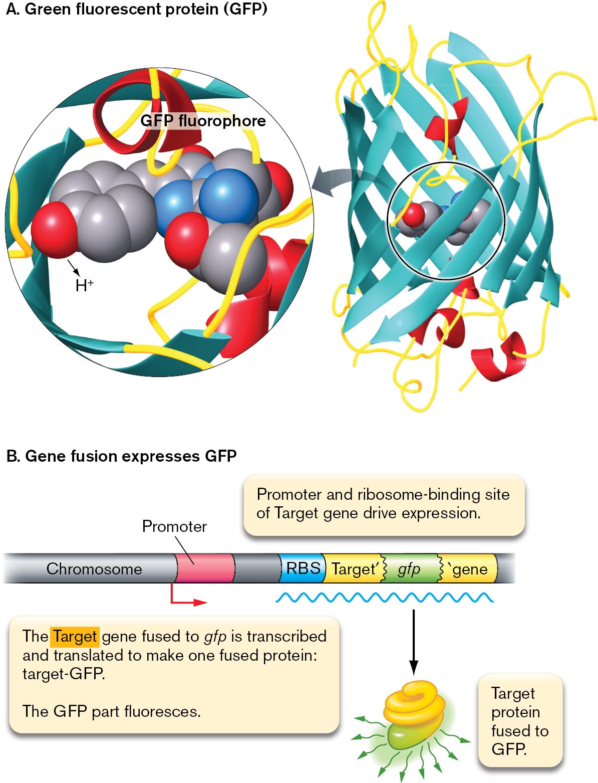
Gene fusion reporter. Cells can be engineered with a gene fusion, a fused gene that expresses a bacterial protein combined with either GFP or one of many GFP variants expressing different colors (Fig. 2.29).
More information
A model of G F P fluorophore and a model of G F P gene fusion.
A space filling model and the protein structure of G F P fluorophore are shown. The protein structure of G F P shows the fluorophore within barrel-shaped beta-sheets. A magnified view of the fluorophore shows a space-filling model of the three amino acids serine, tyrosine, and glycine, bonded.
A model of G F P gene fusion. A chromosome sequence has the promoter, R B S, target gene prime, g f p, and prime gene. An arrow points forward from the promoter, and an m R N A strand lies below the chromosome. From the m R N A strand, an arrow points down to show a truncated protein fused with another protein fluorescing. The fused protein is labeled, target protein fused to G F P. Accompanying text reads, The target gene fused to g f p is transcribed and translated to make one fused protein: target hyphen G F P. The G F P part fluoresces. Above the chromosome sequence, text reads, promoter and ribosome binding site of target gene drive expression.
FIGURE 2.29 ■The fluorophore green fluorescent protein (GFP).A. Green fluorescent protein (GFP) is expressed endogenously by the cell. Blowup: Three GFP amino acid residues (serine, tyrosine, and glycine) condense to form the fluorophore. B. The gene encoding GFP can be fused to a target gene (Target′-gfp). The fused gene then expresses a fused protein in which the GFP portion fluoresces. The fluorescent protein is expressed under control of the target gene promoter and ribosome-binding site (RBS).
Originally isolated from a jellyfish (Aequorea victoria), the Nobel Prize–winning GFP can be expressed from a gene spliced into the DNA of any organism; even monkeys have been engineered to glow green. How does GFP act as a fluorophore? The fluorophore part of GFP consists of three amino acid residues that react to form an aromatic ring structure, embedded within a beta barrel protein tube. The properties of the fluorophore are modified by the surrounding protein, so mutation of the gene encoding GFP generates numerous variants with different spectral ranges.
Remarkably, GFP and related fluorescent proteins can be modified as markers of specific target proteins of interest in a cell. This modification is called a gene fusion (Fig. 2.29). A gene fusion consists of a target gene fused to a gene encoding GFP, which gets expressed via the target control sequences and translated by ribosomes using the target ribosome-binding site (RBS). The fused protein can fluoresce as a marker pinpointing the position of the target protein within the cell (Fig. 2.29B). The target protein function may be surprisingly normal, despite the fused GFP.
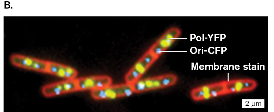
The wide range of colors of GFP variants provides an extraordinary set of probes for the internal structure of a cell. For example, different fluorophores label specific molecules during DNA replication within a growing cell of Bacillus subtilis (Fig. 2.30B). The red color arises from the membrane-specific fluorophore FM4-64. The DNA origin of replication is labeled blue by cyan fluorescent protein (CFP), a color variant of GFP. The gene encoding CFP is fused to a gene encoding a DNA-binding protein specific to the B. subtilis origin of replication. The replisomes (DNA polymerases) are labeled yellow, owing to a fused gene encoding yellow fluorescent protein (YFP). The replisomes usually locate together near the center of the cell, but sometimes they separate and are visible as two yellow spots.
Another exciting application is that GFP and related protein fluorophores can be engineered to report chemical conditions within a cell. For example, the ionized and protonated forms of GFP (labeled in Fig. 2.29A) have slightly different excitation ranges, thus affording a way to measure hydronium ion concentration (pH) within a cell. This property enables GFP to report on a cell’s response to pH stress. Other GFP sensors are designed to report concentrations of chloride or calcium, second messengers, redox level, or even protease activity.
Thought Question
2.6 What experiment could you devise to determine the order of events in Bacillus subtilis DNA replication?
ANSWER ANSWER
One way to track the movement of DNA during DNA replication would be to stain the DNA with a dye such as DAPI at various stages of cell division. Alternatively, green fluorescent protein (GFP) fused to a DNA-binding protein could be used to label a specific sequence of DNA and track its position. A way to determine the order of events in sporulation could be to observe mutant strains of bacteria that contain defects in different proteins of the replication process. (DNA replication is discussed further in Chapter 7.)
A concern with the use of GFP fluorescence is that proteins fused to GFP may behave differently from the original nonfused protein. In some cases, the GFP portion causes fusion proteins to form complexes at the cell poles that are absent in non-GFP cells. Thus, in cellular biology it is always important to confirm data with the results of a different kind of technique; for example, localization of the target protein with a labeled antibody.
Note also in Figure 2.30B that the labeled membranes and DNA origin appear diffuse; that is, unresolved. The emitted light travels in all directions from the point source of the object, and its resolution is limited by the wavelength. Thus, fluorescence cannot resolve the detailed shape of a protein or distinguish two proteins that are close together. But we can detect the location of a DNA-binding protein within a cell and resolve it as distinct from another fluorescent object located elsewhere. Furthermore, computational techniques called super-resolution imaging enable us to pinpoint the protein’s location with a precision tenfold greater than the resolution of ordinary optical microscopy.
More information
A photo of a scientist using a fluorescence microscope and a fluorescence micrograph are shown.
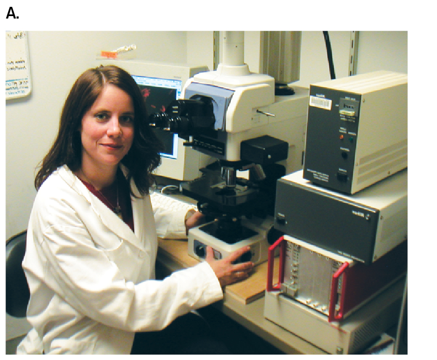
A photo shows Melanie Berkmen using a fluorescence microscope.
More information
A fluorescence micrograph of the D N A origin of replication. The fluorescence micrograph shows five rod-shaped cells, each about 4 micrometers long. The labeled parts are Pol-Y F P which is yellow, O r i-C F P which is blue, and membrane stain which is red.
FIGURE 2.30 ■The replisome and the DNA origin of replication.A. Melanie Berkmen, working in the laboratory of Alan Grossman, obtains the fluorescence micrograph shown in panel B. B. Fluorescence microscopy reveals the DNA origin, labeled blue by a protein fused to cyan fluorescent protein, binding at a sequence near the origin (Ori-CFP). Replisomes are labeled yellow by fusion of a DNA polymerase subunit to yellow fluorescent protein (Pol-YFP) in dividing cells of Bacillus subtilis.COURTESY OF MELANIE BERKMEN, MITCOURTESY OF MELANIE BERKMEN, MIT
Super-Resolution Imaging
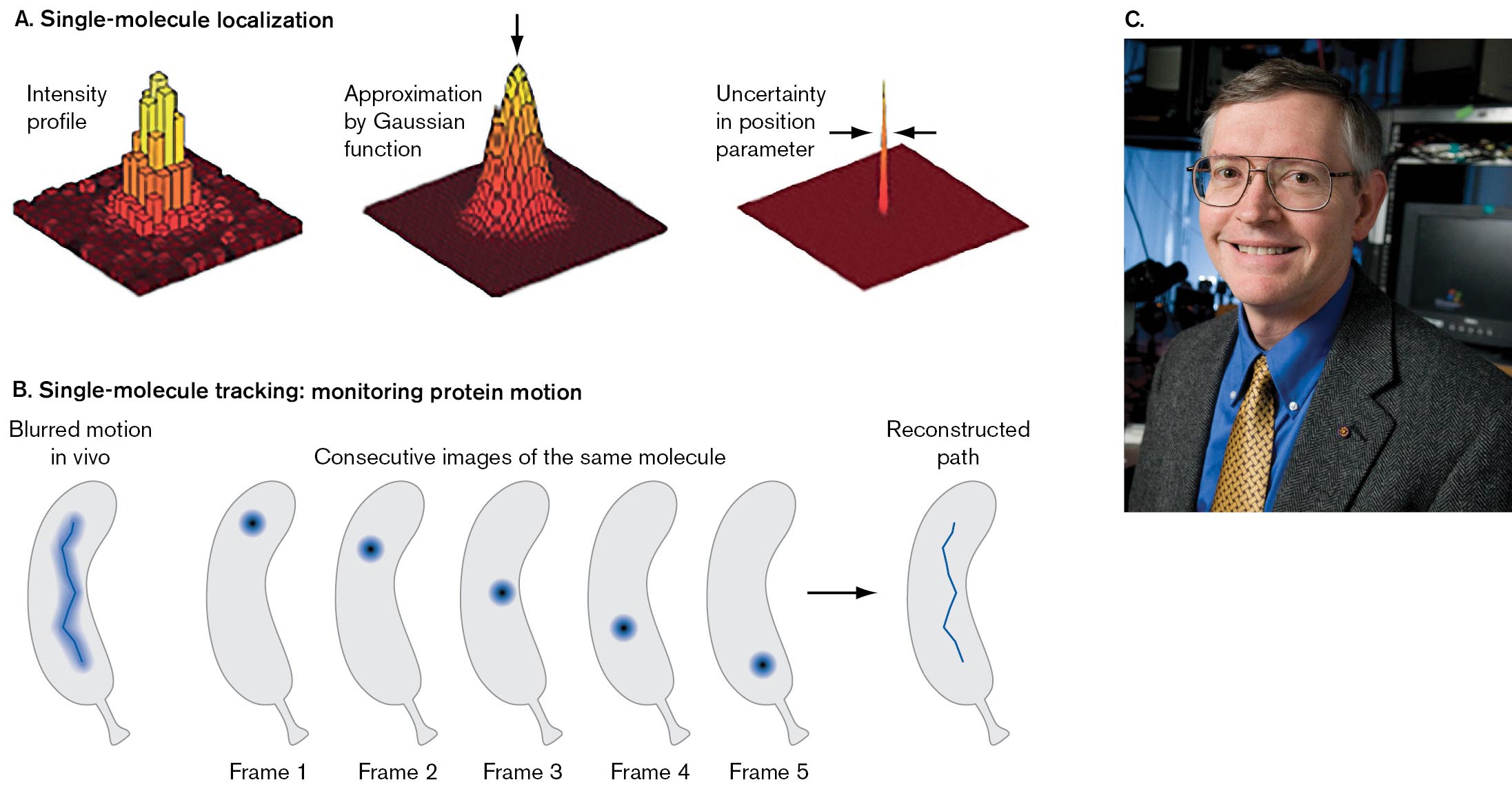
Cell function requires the interaction of key single molecules, such as the chromosomal DNA with a protein binding its origin. William Moerner at Stanford University was the first to demonstrate the possibility of single-molecule tracking of fluorescent proteins in bacteria (Fig. 2.31). The 2014 Nobel Prize in Chemistry honored Eric Betzig, Stefan Hell, and William Moerner for the development of super-resolved fluorescence microscopy, or super-resolution imaging.
More information
Two illustrations describe single-molecule localization. A photo of William Moerner accompanies the illustrations.
An illustration depicts single-molecule localization. It consists of three diagrams. The first diagram shows the three-dimensional plane in which the building blocks of the peak are positioned in the center, and the corresponding text reads intensity profile. The second diagram shows a smoother peak positioned in the center of the plane. A down arrow points at the peak from the top. The corresponding text reads approximation by Gaussian function. The third diagram shows a narrow peak at the center of the plane, and the corresponding text reads uncertainty in the position parameter.
An illustration of single-molecule tracking: monitoring protein motion. It shows six bean-shaped images representing cells. The image at the left, a blurred zig-zag line inside the cell is labeled as blurred motion in vivo. The other five images are labeled as frame 1, frame, 2, frame 3, frame 4, and frame 5. The five frames are collectively labeled consecutive images of the same molecule. Dot shaped molecules are present inside the cell at a different position. The frame 5 leads to a sharp zig-zag line inside a cell labeled as reconstructed path.
A photo shows William Moerner.
FIGURE 2.31 ■Single-molecule localization by computation: a form of super-resolution imaging.A. The uncertainty of the central peak position. B. Tracking a single molecule in a cell. C. William Moerner was the first to demonstrate the possibility of single-molecule tracking of fluorescent proteins in bacteria.ANDREAS GAHLMANN AND WILLIAM MOERNER. 2014. NAT. REV. MICROBIOL. 12:9LINDA A. CICERO/STANFORD NEWS
How can we track a single molecule, which is far smaller than the resolution limit of light (λ/2 = 200 nm)? Recall the shape of the magnified image of a point source of light (Fig. 2.12). Upon magnification, each image of a point source appears as a peak intensity surrounded by rings of much lower intensity. The sharpness of the main peak is limited by the wavelength of light. But the precision with which we know the peak’s central position is much narrower (Fig. 2.31A). In other words, the uncertainty of the central peak position is about a tenth the width of the intensity profile. Computation based on the intensity profile can reveal the peak positions with high precision. The peak positions show how individual proteins move within a living cell (Fig. 2.31B).
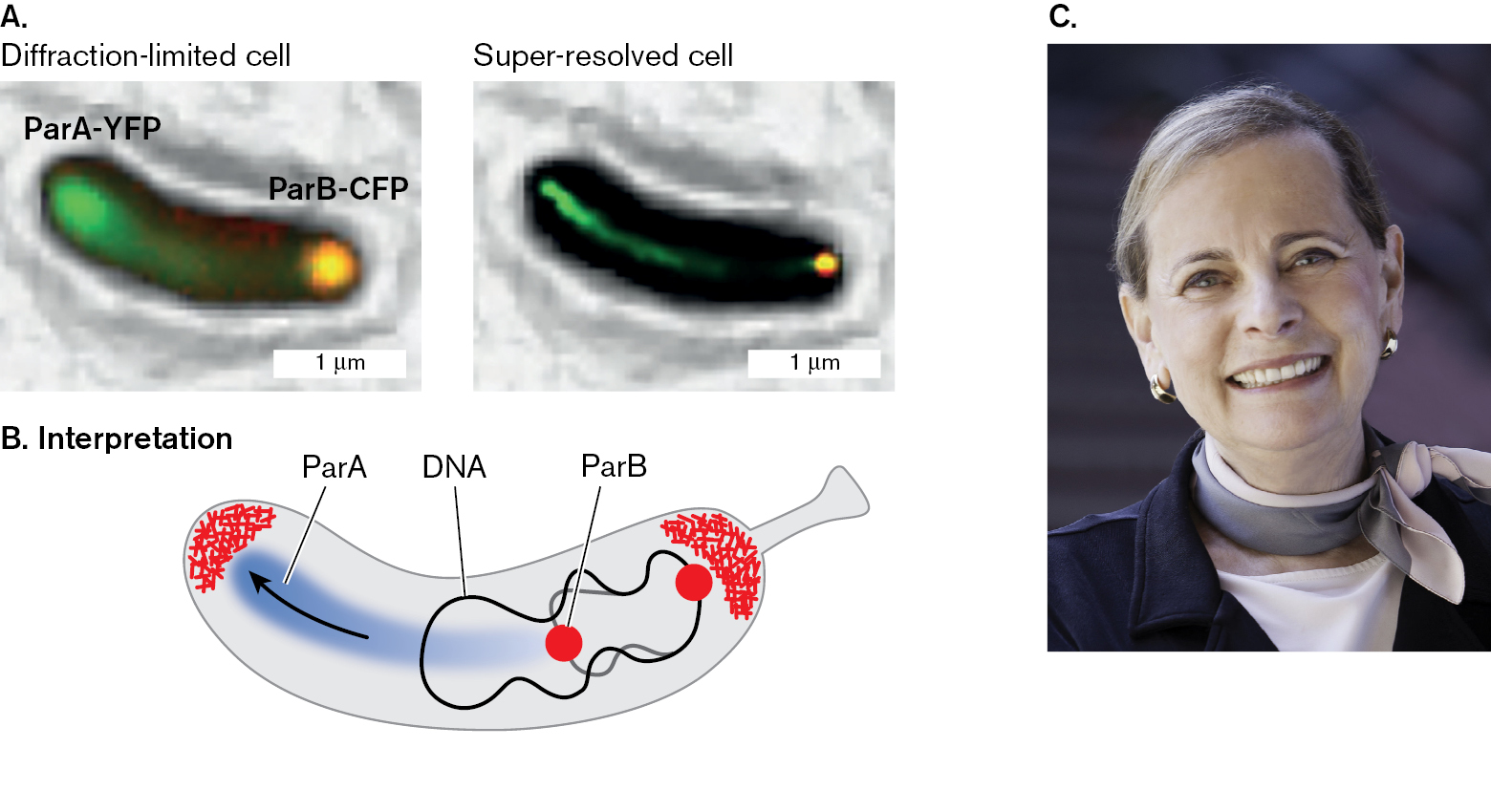
In an early application of super-resolution imaging, Moerner worked with Lucy Shapiro at Stanford University to track the movement of DNA-binding proteins during cell fission of Caulobacter crescentus (Fig. 2.32). Shapiro received the National Medal of Science from President Obama in 2013 for her studies of the intriguing developmental cycle of this bacterium, which involves a transition between stalked and flagellar cells (presented in Chapter 3). Moerner, Shapiro, and their students used super-resolution imaging to track the migration of the ParA cell fission protein (Fig. 2.32A and B). In this experiment, the gene encoding ParA is fused to a gene for yellow fluorescent protein (YFP), whereas the gene encoding ParB is fused to a gene for cyan fluorescent protein (CFP). The ParA protein migrates clear across the cell, generating a spindle-like track to guide the ParB protein as it pulls the newly replicated DNA origin from one pole to the opposite pole. Many similar intracellular mechanisms are explored in Chapter 3.
More information
Two super resolution images of origin binding proteins, an illustrated interpretation, and a photo of Lucy Shapiro.
Two super resolution images of origin binding proteins in Caulobacter crescentus. Both images contain a rod shaped cell of 3 micrometers in length and 0.5 micrometer in width. The first image is labeled diffraction-limited cell. The cell in this image is labeled as Par A-Y F P at the top end and Par B-C F P at the bottom end. The second image is labeled super-resolved cell. The cell in this image is labeled as Par A-Y F P at the top end and Par B-C F P at the bottom end
An illustrated interpretation of Par A protein migration through a cell. Within the cell, there are dots attached to a twisting strand of D N A. The dots are labeled as Par B. A group of molecules collect at the left and the right of the cell. An arrow labeled Par A points from Par B towards the group of molecules at the left of the cell.
A photo of Lucy Shapiro.
FIGURE 2.32 ■Super-resolution imaging reveals movement of origin-binding proteins across a cell.A. Super-resolution imaging reveals the migration of the ParA cell fission protein across the cell of Caulobacter crescentus. The gene encoding ParA is fused to a gene encoding YFP, and the gene encoding ParB is fused to a gene encoding CFP. B. The ParA protein migrates clear across the cell, generating a track to guide the ParB protein as it pulls the newly replicated DNA origin across from one pole to the opposite pole. The arrow indicates movement. C. Lucy Shapiro, winner of the National Medal of Science in 2013.JEROD L. PTACIN ET AL. 2010. NAT. CELL BIOL. 12:791LUCY SHAPIRO
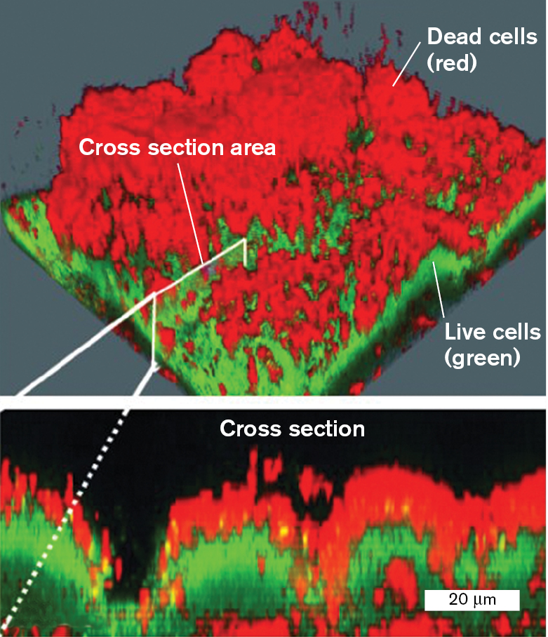
Some advanced forms of fluorescence microscopy use laser beams to resolve subcellular details, and even to visualize cells in 3D. One such method is confocal laser scanning microscopy (or confocal microscopy). In confocal microscopy, a microscopic laser light source scans across the specimen. Figure 2.33 shows a biofilm composed of the pathogenic bacterium Pseudomonas aeruginosa treated with the antibiotic tobramycin. The biofilm is treated with fluorophores that reveal live cells (green) beneath the dead cells killed by tobramycin (red). The hidden live cells cause problems for medical therapy. Confocal microscopy enables us to visualize the 3D structure of the biofilm. The method of confocal microscopy is explained in eAppendix 3.
More information
Two confocal laser scanning micrographs show the observation of a biofilms with live and dead cells containing a fluorophore. The laser scanning electron micrographs show a rough biofilm surface. The live cells fluoresce green at the bottom layer, and the dead cells fluoresce red at the top layer. The area between the dead and live cells is labeled as a cross-section. A micrograph of the cross-section shows the layering in greater detail with red on the top and bottom and green in the middle.
FIGURE 2.33 ■Biofilm with live/dead fluorophore, observed by confocal laser scanning microscopy.Pseudomonas aeruginosa cells growing in a biofilm treated with the antibiotic tobramycin. Dead cells fluoresce red; live cells fluoresce green.MORTEN HENTZER AND MICHAEL GIVSKOV. 2003. J. CLIN. INVEST.112:1300
Confocal imaging can be used for 3D imaging of pathogens embedded within host cells or tissue. We saw an example in the chapter-opening image, where infective Salmonella cells were observed within intracellular vesicles. Another advanced form of fluorescence imaging involves the CLARITY technique. This remarkable method generates optical clarity in background tissue, revealing the spatial distribution of bacteria that colonize a host tissue (see Special Topic 2).
Fluorescence In Situ Hybridization (FISH)
Fluorescent labeling can be used to show the spatial location of microbial taxa. This technique is fluorescence in situ hybridization, or FISH. FISH can map specific taxa of microbes within an environment such as soil or within a host organ such as the human intestinal epithelium.
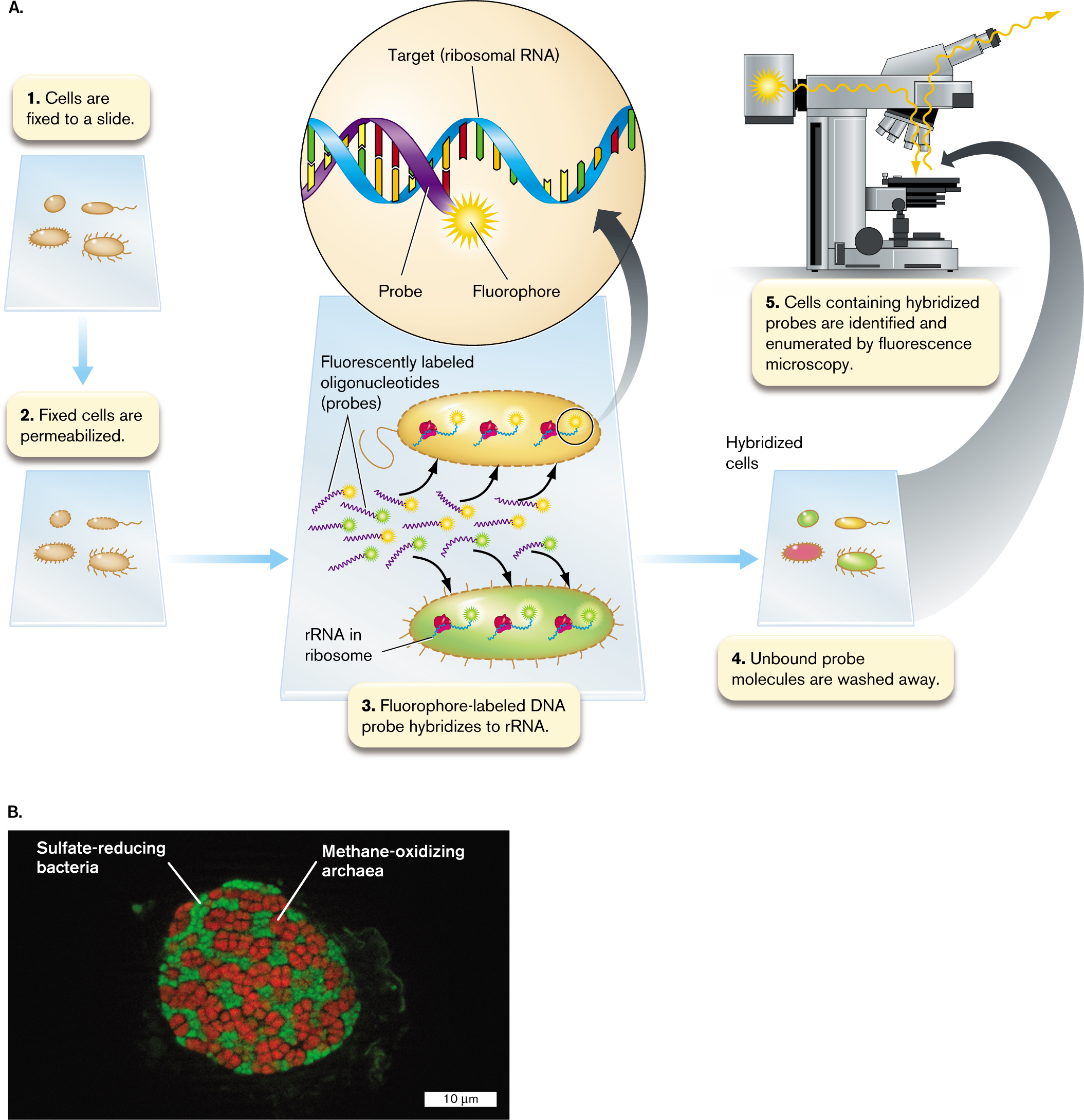
The FISH technique (Fig. 2.34A) makes use of a fluorophore-labeled oligonucleotide probe (usually a short DNA sequence) that hybridizes to a microbe’s DNA or ribosomal RNA (rRNA). Hybridizing to rRNA increases sensitivity because rRNA is present in approximately 100-fold to 10,000-fold excess over DNA.
In a typical procedure, the cells of a sample are fixed to a slide (Fig. 2.34A, step 1) by a chemical treatment that maintains cell integrity while permeabilizing the cell so that the fluorophore-labeled DNA probe can enter (step 2). Next the fixed cells are incubated in a hybridization buffer containing the probe, at a temperature designed to maximize specificity of binding to the sequence of the desired taxa (step 3). A probe with broad specificity might hybridize to all bacterial rRNA, but not to archaeal or eukaryotic rRNAs. For greater specificity, a probe may have a sequence complementary to a sequence found only in rRNA of a given bacterial taxon. After hybridization and a wash (step 4), the cells containing hybridized probes are observed by fluorescence microscopy (step 5).
SPECIAL TOPIC 2Biogeography of a Gut Pathogen
What do microbial pathogens really look like within the host organ they infect? The host tissue constitutes a vast geography, where the microbe’s location may determine its ability to cause disease. William DePas (Fig. ST 2.1A), in the laboratory of Dianne Newman at the California Institute of Technology, combined several state-of-the-art technologies to image the biogeography of pathogens. Ana Hernandez-Gallego (Fig. ST 2.1B) with Fitnat Yildiz, at UC Santa Cruz, used the method to study virulence factors of the pathogen Vibrio cholerae during infection of the mouse gut.
More information
A photo of William DePas and a photo of Ana Hernandez-Gallego.
A photo of William DePas.
More information
A photo of Ana Hernandez-Gallego.
FIGURE ST 2.1 ■William DePas and Ana Hernandez-Gallego. DePas developed the MiPACT technique, and Hernandez-Gallego applied it to study the virulence of Vibrio cholerae during mouse infection.COURTESY OF WILLIAM DEPASANA LUCÍA GALLEGO HERNÁNDEZ
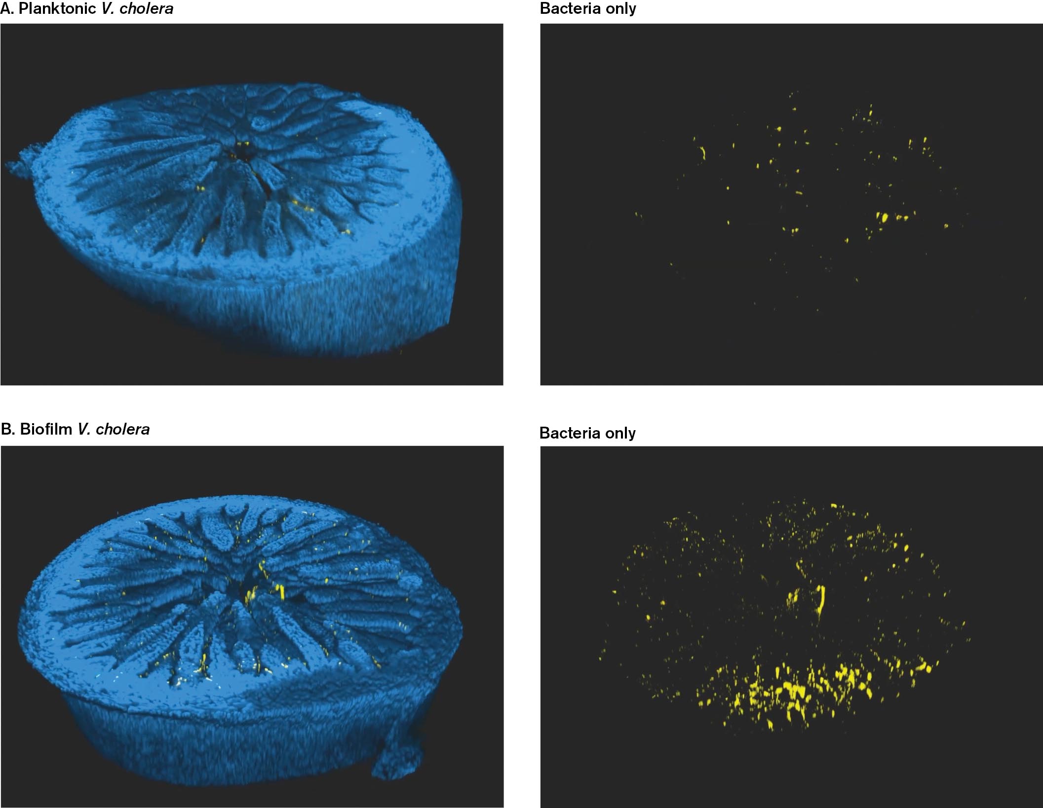
The first technology used is the CLARITY technique, which can render tissues transparent for whole organs. The technique selectively removes the tissue’s lipid components, which are the main cause of opacity. DePas devised MiPACT, a microscale version of CLARITY that allows microscopic visualization of cells within a tissue section (Fig. ST 2.2). The mouse cells are labeled blue with DAPI fluorophore bound to nuclear DNA, whereas the bacteria are labeled yellow by a fluorophore attached to a DNA probe that hybridizes to the bacterial chromosome.
More information
Four MiPACT images of planktonic and biofilm Vibrio cholerae within the mouse gut epithelium.
MiPACT imaging of planktonic Vibrio cholerae within the mouse gut epithelium. A large blue section of the nuclei of villi is seen. A few tiny yellow dots of V. cholerae cells are visible.
MiPACT imaging of planktonic Vibrio cholerae. Several loosely connected yellow cells of V. cholerae are visible. The image is labeled bacteria only.
MiPACT imaging of biofilm Vibrio cholerae within the mouse gut epithelium. A large blue section of the nuclei of villi is seen. Several yellow clumps of V. cholerae cells are visible.
MiPACT imaging of biofilm Vibrio cholerae. A large number of yellow V. cholerae cells are visible. The image is labeled bacteria only.
FIGURE ST 2.2 ■MiPACT imaging reveals Vibrio cholerae within the mouse gut epithelium. Mouse intestinal sections were made transparent. DAPI (blue) stains nuclei of villi. Vibrio cholerae (yellow) are identified by the hybridization chain reaction (HCR). Inoculated cells were A. planktonic, see video; B. biofilm, see video. (Panel A: ; Panel B: )A. L. GALLEGO HERNÁNDEZ. 2020. PROC NATL ACAD SCI USA. 117:11010–11017A. L. GALLEGO HERNÁNDEZ. 2020. PROC NATL ACAD SCI USA. 117:11010–11017A. L. GALLEGO HERNÁNDEZ. 2020. PROC NATL ACAD SCI USA. 117:11010–11017A. L. GALLEGO HERNÁNDEZ. 2020. PROC NATL ACAD SCI USA. 117:11010–11017
Planktonic V. cholerae colonization of mouse intestine
Biofilm V. cholerae colonization of mouse intestine
To render the tissue transparent, the sample is soaked in acrylamide monomers that cross-link with each other and with the protein components of the tissue. The lipid components are then dissolved by sodium dodecyl sulfate (SDS) detergent, the same detergent used for gel electrophoresis. Once the tissue clears, a final solution treatment removes the SDS and adds a preservative chemical. The clarified tissue retains structural proteins as well as DNA. A lysozyme treatment then breaks down bacterial cell walls, enabling the entry of DNA-hybridizing probes. To detect specific types of bacteria, DePas used an advanced version of FISH called the hybridization chain reaction (HCR). In this technique, specific bacteria are detected by hybridization of their RNA with a species-specific DNA probe. The hybridization reaction activates multiple fluorophores, magnifying the signal.
The MiPACT technique reveals the presence of V. cholerae bacteria within the landscape of mouse intestinal villi. Hernandez-Gallego used this technique to compare the colonization ability of V. cholerae from populations that were grown as planktonic (Fig. ST 2.2A) or as biofilm (Fig. ST 2.2B). After mouse infection, sections of colon are obtained. The bacteria are visualized by HCR as yellow, whereas the nuclei of intestinal villi are stained blue with DAPI fluorophore; their surrounding cytoplasm is transparent. Individual V. cholerae cells can be counted, revealing that biofilm-grown populations show increased colonization. The movies rotate through each section, showing the distribution of the pathogen. This technique enables us to study the process of infection in unprecedented detail.
RESEARCH QUESTION
How can we use MiPACT imaging to study the mechanism and effectiveness of antibiotic therapies on host infections?
Gallego-Hernandez, A. L., W. H. DePas, J. H. Park, J. K. Teschler, R. Hartmann, et al. 2020. Upregulation of virulence genes promotes Vibrio cholerae biofilm hyperinfectivity. Proceedings of the National Academy of Sciences USA117:11010–11017.
Note: For microbial ecology, FISH usually involves probe hybridization to ribosomal RNA molecules, whereas for eukaryotic cells the probe is hybridized to a gene on chromosomal DNA.
Figure 2.34B shows an example of FISH used to reveal the deep-sea methanotrophic consortium that oxidizes 90% of the methane emitted by methanogens—a major contribution to the global climate (discussed in Chapter 22). The target community consists of a mixed biofilm of anaerobic methane-oxidizing archaea (ANME) and sulfate-reducing bacteria (SRB), obtained from a methane seep located 2 km below sea level at the Guaymas Basin in the Gulf of California. The biofilm was labeled with oligonucleotide fluorescent probes specific for ANME (red) and for SRB (green).
More information
A diagram of fluorescence in situ hybridization and a micrograph containing fluorescently labeled bacteria and archaea.
A schematic diagram of fluorescence in situ hybridization with five steps. Step 1: Cells are fixed to a slide. Four oval-shaped bacteria are shown on a glass slide. Step 2: Fixed cells are permeabilized. The same slide is shown. Step 3: Fluorophore-labeled D N A probe hybridizes to r R N A. The illustration shows the bacteria taking in fluorescently labeled oligonucleotides, or probes. Each bacterium takes up probes with differently colored fluorophores. The probes hybridize to the r R N A target within the cells. Step 4: Unbound probe molecules are washed away, leaving hybridized cells. The bacteria are shown on the slide with different color profiles. Step 5: Cells containing hybridized probes are identified and enumerated by fluorescence microscopy. The slide is shown on the stage of a fluorescence microscope.
A micrograph of fluorescently labeled methane-oxidizing archaea and sulfate-reducing bacteria. The archaea fluoresce red and the bacteria fluoresce green. The bacteria and archaea are clumped together in a circular unit of about 20 micrometers in diameter.
FIGURE 2.34 ■Fluorescence in situ hybridization (FISH) of bacteria and archaea.A. Fluorophore-labeled DNA oligonucleotide hybridizes to a taxon-specific sequence of rRNA molecules within the cells that are fixed and permeabilized on a microscope slide. B. Syntrophy between anaerobic methane-oxidizing archaea (red FISH) and sulfate-reducing bacteria (green FISH) from a deep-sea cold seep at Guaymas Basin in the Gulf of California.
Source: Part A modified from Rudolf Amann and Bernhard M. Fuchs. 2008. Nat. Rev. Microbiol.6:339, fig. 1.
P. CRUAUD & A. VIGNERON, IFREMER
The FISH image shows the two kinds of cells grouped together in a remarkably regular pattern. The ANME, which extract electrons from methane, thereby releasing CO2, tend to be buried within the sample, surrounded by the SRB. The SRB receive electrons from the ANME and transfer electrons to sulfate, which is reduced to sulfide. Sulfate is a relatively poor electron acceptor (as discussed in Chapter 14), but its high concentration in seawater increases its free-energy contribution (discussed in Chapter 13). The spatial organization of ANME and SRB cells thus facilitates their syntrophy, a form of metabolism in which each partner completes half of a reaction with an overall negative value of ΔG (see Chapter 13). Tight association of the ANME with the sulfate-reducing bacteria enables ANME to transfer electrons from methane directly to the SRB.
Chemical Imaging Microscopy
Chemical imaging uses mass spectrometry (analysis of molecular fragments by mass) to visualize the distribution of chemicals within living cells. The combination of fluorescence and chemical imaging offers extraordinary opportunities to map the structure and function of cells in natural communities, such as soil or the intestinal microbiome.
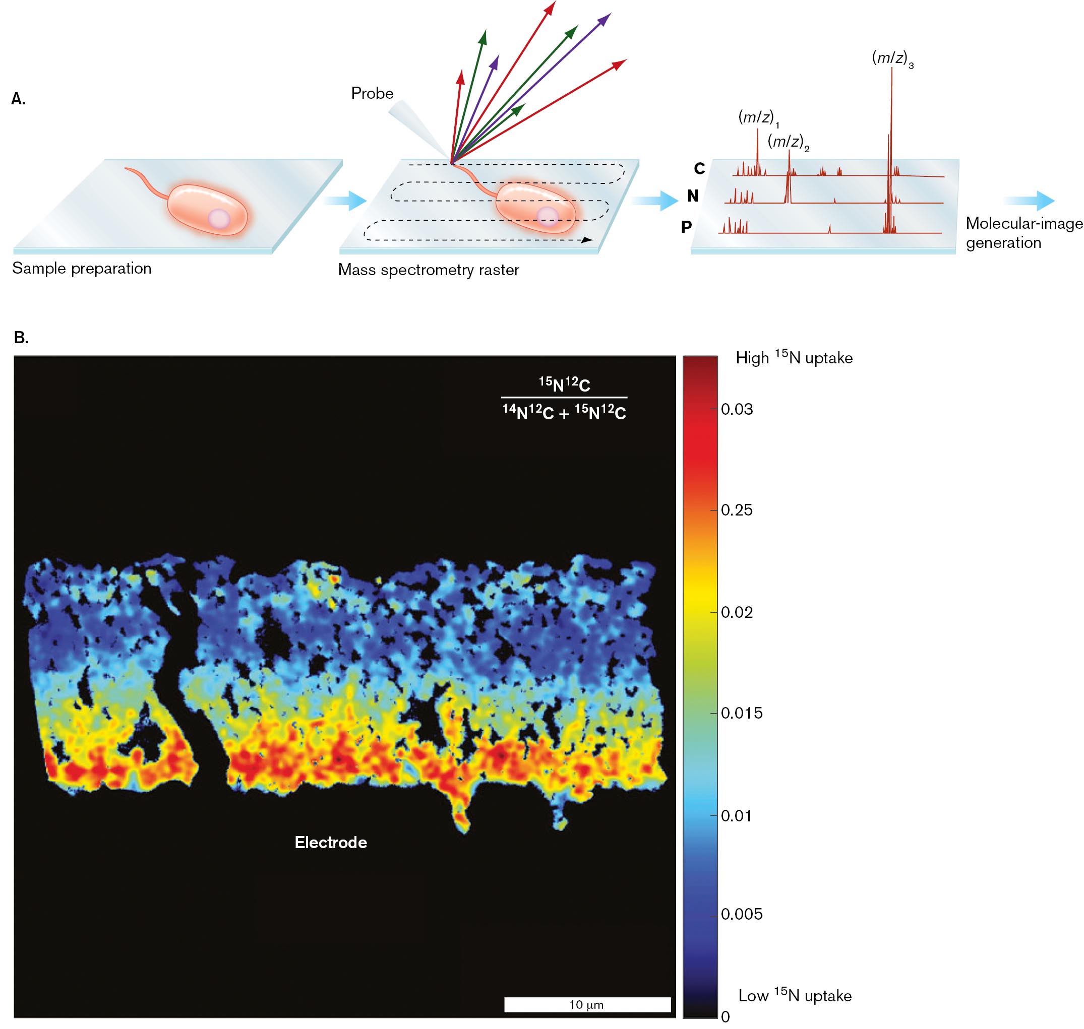
A high-resolution method for chemical imaging is called nanoscale secondary ion mass spectrometry (NanoSIMS). The NanoSIMS process starts with an ionizing probe, a source of energy that breaks up the large organic molecules of a sample (Fig. 2.35A). The molecular fragments, called “secondary ions,” fly off from the source and are captured by a mass spectrometer. This instrument measures fragment masses of the secondary ions, generating a mass spectrum. Mass spectra are taken from thousands of locations, scanned across a bacterial cell.
For NanoSIMS, the microbial sample is prepared by growth on nutrients labeled with a heavy isotope. For example, the cell’s uptake of nitrogen-rich protein can be detected by incorporation of the heavy isotope 15N. The increased weight of 15N compared to the normally predominant 14N (as indicated by the mass ratio 15N/14N) is detected quantitatively in the molecular-fragment masses. Alternatively, we can detect isotopes of carbon (13C/12C) or other isotopes.
Figure 2.35B shows NanoSIMS applied to a biofilm of Geobacter sulfurreducens growing upon an anode (positively charged electrode). The bacteria donate electrons to the electrode, generating electricity for a fuel cell. To optimize performance of the fuel cell, the researchers determined the pattern of metabolic efficiency within the biofilm. (Bacterial electricity is discussed in Chapter 14.) To measure biomass production, the researchers used NanoSIMS to indicate the proportion of uptake of 15N. The 15N fraction—that is, 15N/(14N + 15N)—is represented by color scale in the heat map. The distribution of 15N shows that bacteria contacting the electrode directly incorporate more nitrogen into biomass than do the bacteria at the outer surface.
More information
An illustration of the process of mass spectrometry molecular-image generation and a Nano S I M S image.
An illustration of the process of mass spectrometry molecular-image generation. The first part shows a planar surface labeled sample preparation containing a single-tailed microbe. The second part shows a mass spectrometry raster that consists of a probe with multiple labeling colors following a dotted curving line across the entirety of the planar surface. The third part shows molecular image generation that consists of three horizontal lines on a plane labeled as C, N, and P. A peak labeled mass to charge subscript 1 is plotted on the left side the line C. A peak labeled mass to charge subscript 2 is plotted on the center of the line N. A tall peak labeled mass to charge subscript 3 is plotted on the right side of the line P.
A Nano S I M S image of atomic percentages of nitrogen incorporated into Geobacter sulfurreducens biomass. A color scale describing nitrogen uptake is shown next to the image. The top of the scale is labeled high superscript 15 N uptake. The bottom of the scale is labeled low superscript 15 N uptake. The top of the scale is red and the bottom of the scale is blue. The scale is starts at 0.03 and decreases by 0.05 until it reaches 0. The Nano S I M S image shows a biofilm of G. sulfurreducens above an electrode. The biofilm is red close to the electrode and blue where it is farther from the electrode. An expression reads superscript 15 N superscript 12 C over superscript 14 N superscript 12 C plus superscript 15 N superscript 12 C.
FIGURE 2.35 ■Imaging mass spectrometry. Mass spectra are obtained from thousands of locations throughout the sample surface.A. Molecular fragments are selected for analysis of mass-to-charge ratio (m/z). Selected isotopes may label specific atoms; for example, C, N, or P. The relative intensities of individual compounds are visualized using false-color gradients. B. NanoSIMS of Geobacter sulfurreducens biofilm upon an electrode, showing atomic percentages of nitrogen (15N) incorporated into biomass.
Source: Part B modified from Grayson Chadwick et al. 2019. PNAS116:20716.
G. L. CHADWICK. 2019. PROC NATL ACAD SCI USA. 116:20716–20724
To Summarize
Fluorescence microscopy uses fluorescence by a fluorophore to reveal specific cells or cell parts.
The specimen absorbs light at one wavelength and then emits light at a longer wavelength. Color filters allow only light in the excitation range to reach the specimen and only emitted light to reach the photodetector.
A fluorophore can label a cell part by chemical affinity for a component such as a membrane, attachment to an antibody stain, or attachment to a short nucleic acid that hybridizes to a DNA sequence.
Fluorescent proteins such as GFP can be fused to a specific protein expressed by the cell. Endogenous GFP-type proteins can track intracellular movement of cell parts and can report environmental stress responses.
Super-resolution imaging can define the position of a fluorescent protein with a precision of 20–40 nm, tenfold better than the resolution limit of light magnification.
Fluorescence in situ hybridization (FISH) uses fluorophore-labeled DNA probes to map the spatial location of microbial taxa in the environment or within a host.
Chemical imaging microscopy maps the distribution of compounds within a cell or a microbial community. NanoSIMS uses mass spectral analysis of bacterial components labeled by heavy isotopes.
The wavelength of light that must be absorbed by a molecule in order for the molecule to fluoresce. It is shorter than the emission wavelength and has higher energy.
In biotechnology, the construction of a recombinant gene composed of portions from two different genes, one of which may be a reporter for gene expression.
Techniques of microscopy that pinpoint the location of an object with a precision greater than the resolution of ordinary optical or fluorescence microscopy.
A type of fluorescence microscopy in which the excitation light from a laser and the emitted light from the specimen are focused together, producing high-resolution images.
A technique to detect individual microbes in an ecological or clinical sample, using a fluorophore-labeled oligonucleotide probe (usually a short DNA sequence) that hybridizes to microbial DNA or rRNA.
A technique of chemical imaging in which an ionizing beam breaks off organic ions from a sample, which fly off the sample and are captured for analysis by a mass spectrometer.
A technique of chemical imaging in which an ionizing beam breaks off organic ions from a sample, which fly off the sample and are captured for analysis by a mass spectrometer.
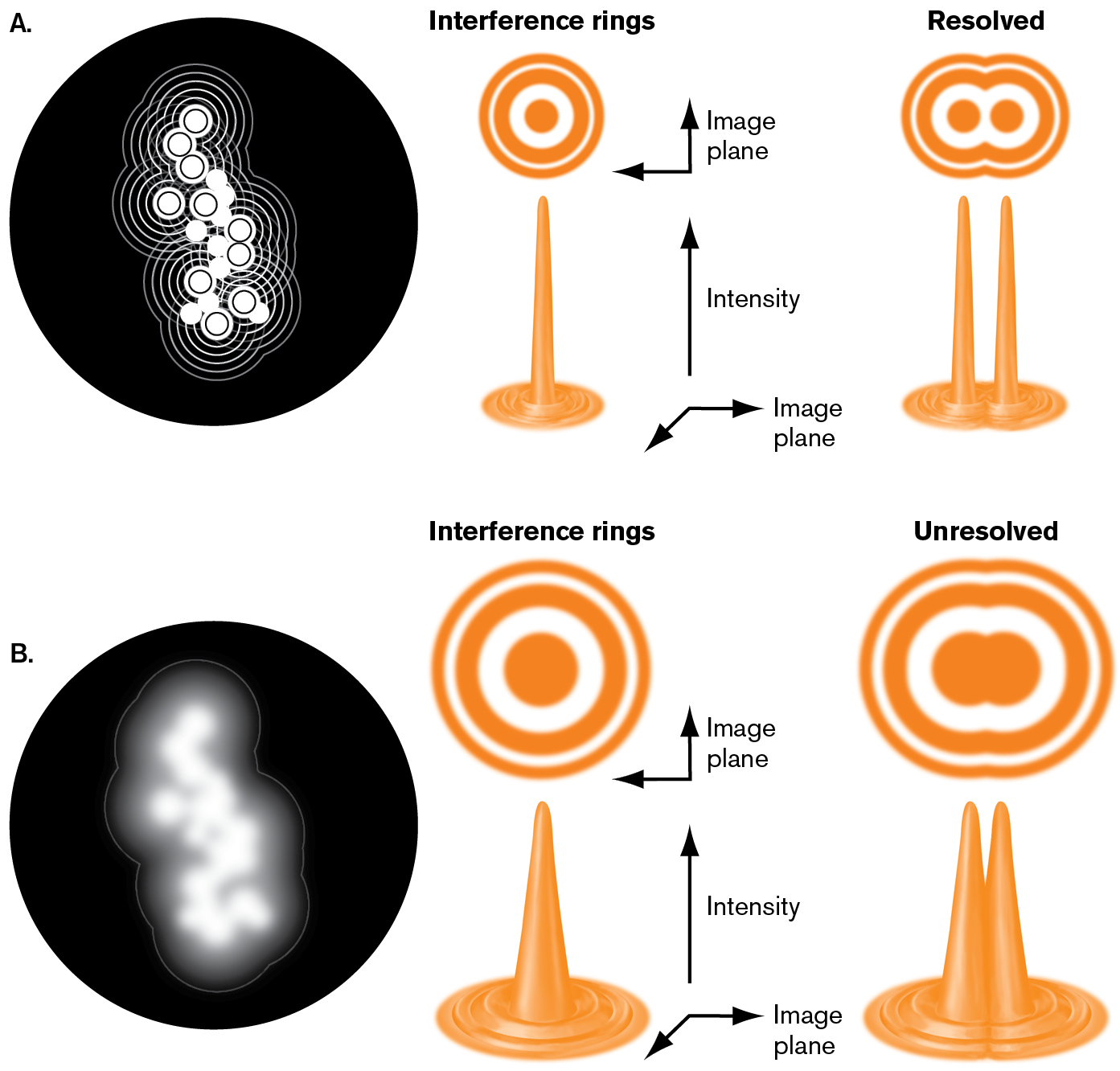
Two illustrations explain interference rings that are resolved versus unresolved.
An illustration depicts narrow interference rings with peaks that are well resolved. It consists of the focal points of light waves that exist in a dark circle. The focal points are represented as lighter dots with distinct ripples. To the right shows the interference rings and resolved rings. The interference rings consist of concentric circles and a bidirectional arrow reads image plane. An image of a narrow peak consists of an upward arrow labeled as intensity, and the bidirectional arrow is labeled as an image plane. In resolved, there are two distinct points that have overlapping concentric rings when viewed in the image plane. When viewed from the side, two distinct narrow peaks are visible.
An illustration depicts wide interference rings with peaks that are unresolved. A large circle with a white shaded region in the center. To the right shows two columns labeled interference rings and unresolved. In the interference ring, a large concentric circle is in the image plane. Below, a wider peak consists of an upward arrow labeled as intensity and a bidirectional arrow labeled as the image plane is at the bottom. In the unresolved example, two circles in the middle overlap and can not be differentiated. Below, two peaks overlap at their bases even though their top points are distinct.
FIGURE 2.12 ■Interference of light waves at the focal point generates concentric rings surrounding the peak intensity.A. Broad wavefronts generate narrow interference rings with peaks well resolved. B. Narrow wavefronts generate wide interference rings that are unresolved.

 ANSWER
 ANSWER