2.6 Electron Microscopy, Scanning Probe Microscopy, and X-Ray Crystallography

Electron Microscopy

How does an electron microscope work? Electrons are ejected from a metal subjected to a voltage potential. Like photons, the electrons travel in a straight line, interact with matter, and carry information about their interaction. And also like photons, electrons can exhibit the properties of waves. The wavelength associated with an electron is 100,000 times smaller than that of a photon; for example, an electron accelerated over a voltage of 100 kilovolts (kV) has a wavelength of 0.0037 nm, compared with 400–750 nm for visible light. However, the actual resolution of electrons in microscopy is limited not by the wavelength, but by the aberrations of the lensing systems used to focus electrons. The magnetic lenses that focus the electrons never achieve the precision required to utilize the full potential resolution of the electron beam.

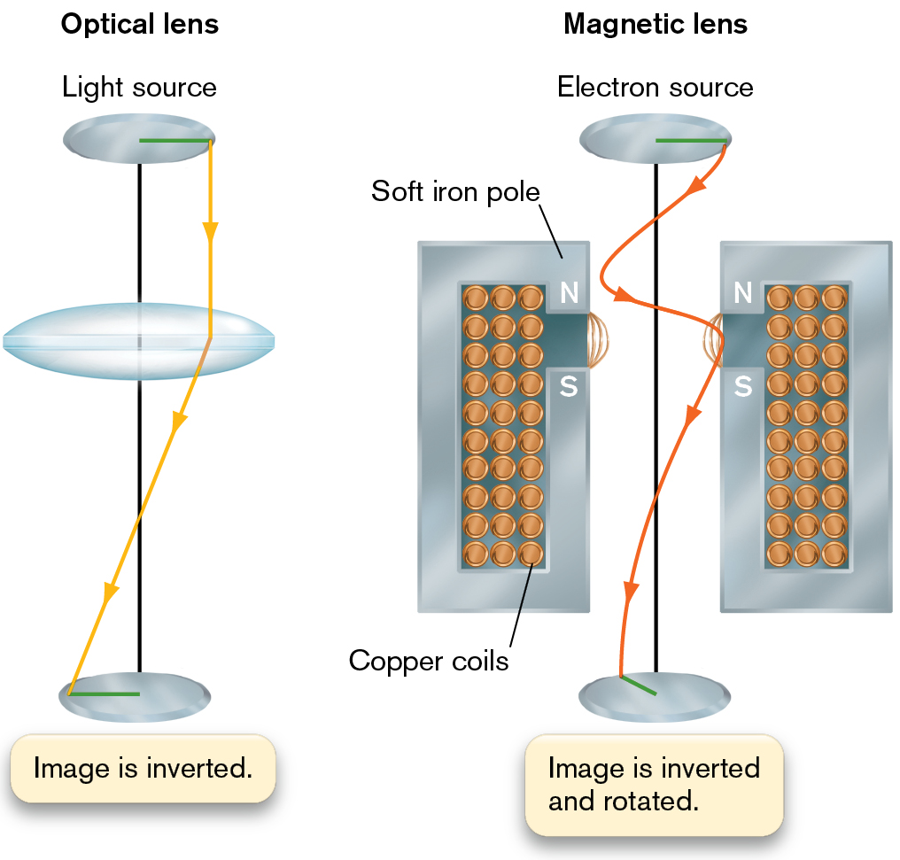
Electrons are focused by means of a magnetic field directed along the line of travel of the beam (Fig. 2.36). As a beam of electrons enters the field, it spirals around the magnetic field lines. The shape of the magnet can be designed to generate field lines that will focus the beam of electrons in a manner analogous to the focusing of photons by a refractive lens. The electron beam, however, forms a spiral because electrons travel around magnetic field lines. Magnetic lenses generate large aberrations; thus, we need a series of corrective magnetic lenses to obtain a resolution of about 0.2 nm. This resolution is a thousand times greater than the 200-nm resolution of light microscopy.

More information

An illustration of an optical lens next to a magnetic lens. The optical lens has a light source at the top. A horizontal line from the center of the lens moves horizontal right. The image is inverted at the bottom of the diagram and the line is now drawn to the left of center. A large concave lens is placed between the light source and the bottom image. An arrow from the right side of the light source falls on the left end of the bottom image after refracting as it passes through the center concave lens. The second part shows the magnetic lens. The electron source is at the top. At the bottom the image is inverted and rotated. A vertical line connects the electron source and the image. Two vertical bars containing several copper coils with the north and south pole labeled as soft iron pole at the left and right of the vertical line. An arrow from the right end of the electron source moves towards one magnet and then the other before reaching the image on the left, rear side of the vertical line.

Thought Question

2.7 Like a light microscope, an electron microscope can be focused at successive powers of magnification. At each level, the image rotates at an angle of several degrees. Given the geometry of the electron beam (see Fig. 2.36), why do you think the image rotates?

ANSWER ANSWER

The image rotates because the electron beam is not straight, as for photons, but travels in a spiral through the magnetic field lines. As magnification increases, the spiral expands, and it reaches the image plane at a slightly different angle than before.

Transmission EM and scanning EM. Two major types of electron microscopy are transmission electron microscopy (TEM) and scanning electron microscopy (SEM). In TEM, electrons are transmitted through the specimen as in light microscopy to reveal internal structure. In SEM, the electron beams scan across the surface of the specimen and are reflected to reveal the contours of its 3D surface.

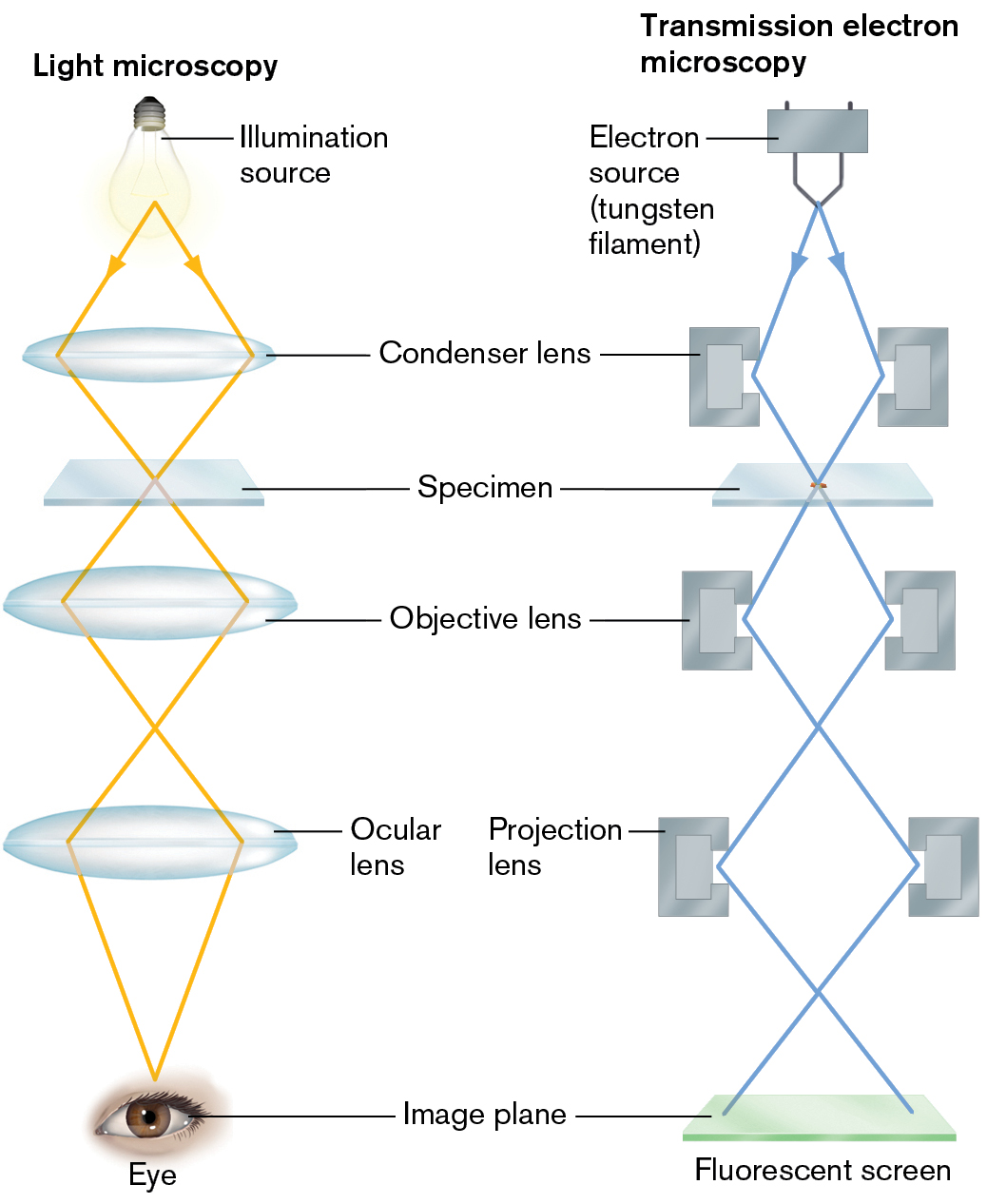
The transmission electron microscope closely parallels the design of a bright-field microscope, including a source of electrons (instead of light), a magnetic condenser lens, a specimen, and a magnetic objective lens (Fig. 2.37). The light source is replaced by an electron source consisting of a high-voltage current applied to a tungsten filament, which gives off electrons when heated. The electron beam is focused onto the specimen by the magnetic condenser lens. The specimen image is then magnified by the magnetic objective lens. The magnetic projection lens, analogous to the ocular lens of a light microscope, focuses the image on a fluorescent screen.

More information

An illustration of light microscopy next to an illustration of transmission electron microscopy. The first illustration shows light microscopy. The light microscopy begins with a bulb labeled as an illumination source. Light is emitted down diagonally, hitting the condenser lens on the far right and far left. The light leaves diagonally moving towards each other, meeting up at the Specimen before leaving in the opposite direction to hit the objective lens on the far left and far right. The light leaves the objective lens moving towards each other, crossing over and moving apart again before hitting the ocular lens on the far left and far right. The light leaves the ocular lens moving towards each other, uniting at the human eyepiece at the bottom.

The second illustration shows transmission electron microscopy begins with an electron source, the tungsten filament. Electrons are emitted down diagonally, hitting the left and right portions of the condenser lens. The electrons leave diagonally moving towards each other, meeting up at the Specimen before leaving in the opposite direction to hit the left and right portion of the objective lens. The electrons leave the objective lens moving towards each other, crossing over and moving apart again before hitting the fluorescent screen, at the bottom.

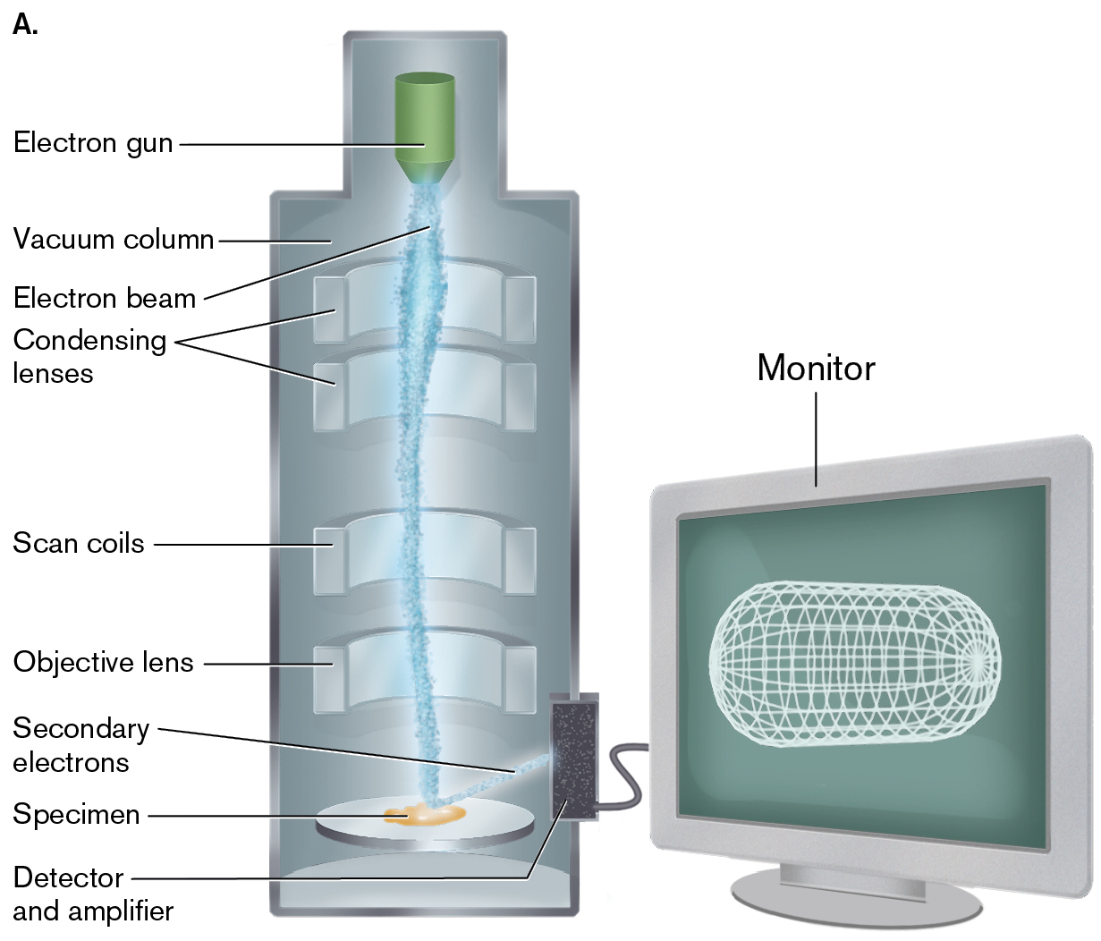
The scanning electron microscope is arranged somewhat differently from the TEM, in that a series of magnetic condenser lenses focuses the electron beam onto the surface of the specimen. Reflected electrons are then picked up by a detector (Fig. 2.38).

More information

An illustration of the structure of a scanning electron microscope and a photo of specimen loading into an S E M.

An illustration of the structure of a scanning electron microscope. The microscope is a cylinder-shaped structure connected to a computer monitor. At the top of the microscope is an electron gun, which sends an electron beam down the microscope to the specimen. The electro beam travels through condensing lenses, scan coils, and an objective lens before it reaches the specimen. A detector and amplifier connects the microscope to the monitor. The side of the amplifier located inside the microscope sends secondary electrons to the specimen. The cylinder structure is labeled as the vacuum column.

More information

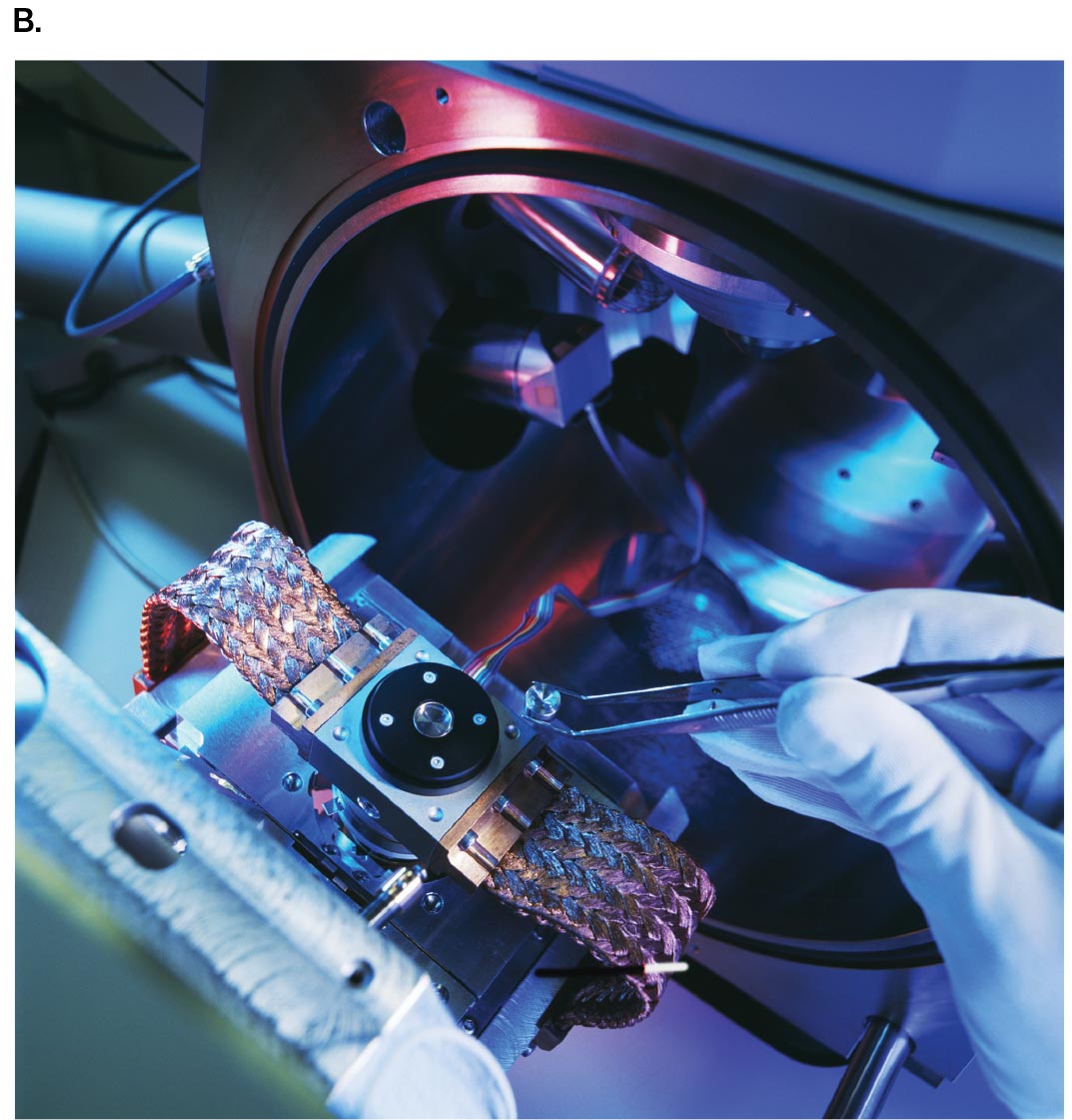
A photo shows a human hand inserting a specimen into the vacuum column of the scanning electron microscope.

Sample preparation for EM. Standard electron microscopy of biological specimens at room temperature poses special problems. The entire optical column must be maintained under vacuum to prevent the electrons from colliding with the gas molecules in air. The requirement for a vacuum precludes the viewing of live specimens, which in any case would be quickly destroyed by the electron beam. Moreover, the structure of most specimens lacks sufficient electron density (ability to scatter electrons) to provide contrast. Thus, the specimen requires an electron-dense negative stain using salts of heavy-metal atoms such as tungsten or uranium. The heavy atoms collect outside the surfaces of cell structures such as membranes, where their electron scatter reveals the outline of the structure. Staining, however, can be avoided for cryo-electron microscopy (discussed next).

We can prepare a specimen by embedding it in a polymer for thin sections. A special knife called a microtome cuts slices through the specimen, each slice a fraction of a micrometer thick. Alternatively, a specimen consisting of, for example, virus particles or isolated organelles can be sprayed onto a copper grid. In either case, the electron beam penetrates the object as if it were transparent. The electrons are actually absorbed by the heavy-atom stain, which collects at the edges of biological structures.

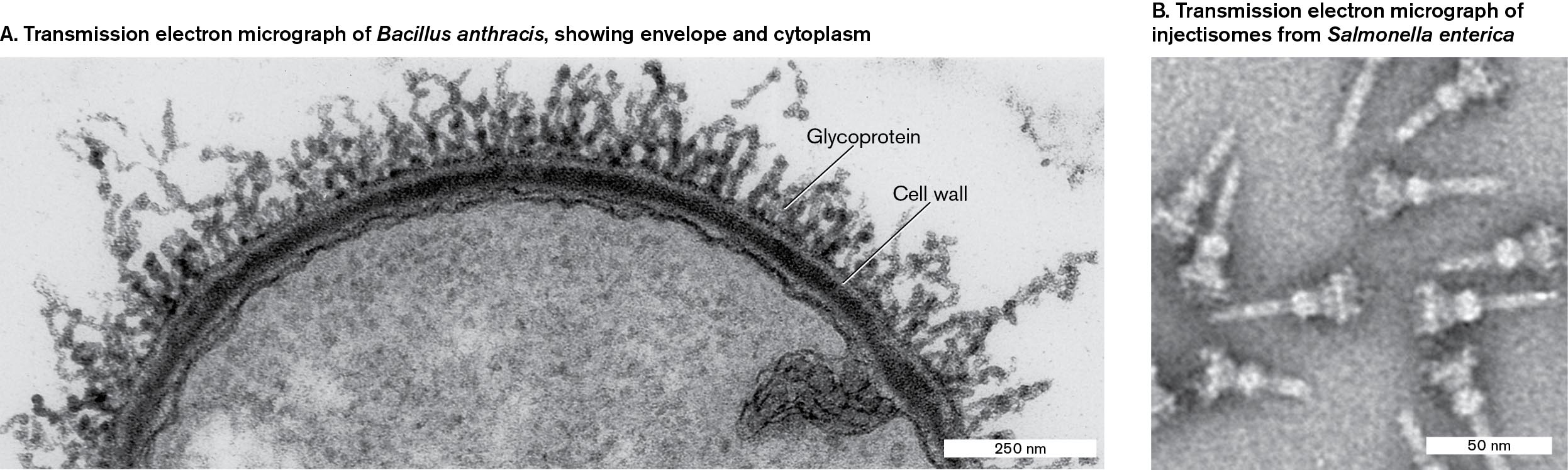
Figure 2.39 shows examples from transmission electron microscopy. The transmission electron micrograph of Bacillus anthracis in Figure 2.39A shows a thin section through a bacillus, including a cell wall, membranes, and glycoprotein filaments. The section is stained with uranyl acetate (a salt of uranium ion). The image includes electron density throughout the depth of the section. In Figure 2.39B, Salmonella protein complexes called “injectisomes” have been isolated and spread on a grid. Injectisomes, or type III secretion systems (T3SS), are used by Salmonella enterica to inject virulence effector proteins into a host cell. The motor protein complexes are negatively stained with phosphotungstate, an electron-dense material that deposits in the crevices around the complexes on the grid. The transmission electron micrograph reveals details of each complex, including the individual rings that anchor it in the cell envelope. The details resolved by the beam of electrons are far smaller than those resolved by a light microscope.

More information

Two transmission electron micrographs of Bacillus anthracis and injectisomes from Salmonella enterica are shown.

A transmission electron micrograph of Bacillus anthracis. It consists of a thin section of Bacillus anthracis, in a semi-circle shape. The structure has a radius of about 500 nanometers. The outer cell is labeled as the cell wall, and the several branching nodules attached to the cell wall are labeled as glycoprotein.

A transmission electron micrograph of injectisomes from Salmonella enterica. It consists of several screw-shaped injectisomes, each about 50 nanometers long.

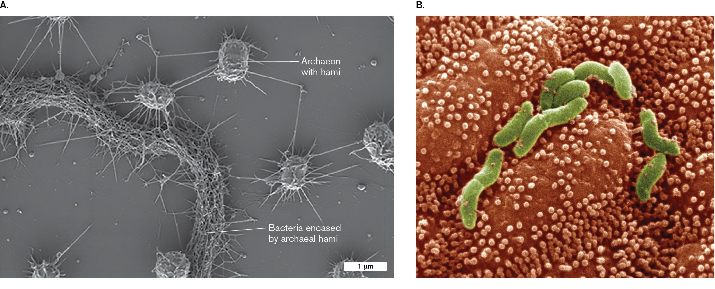
Scanning electron microscopy can show whole cells in apparent 3D view, with much greater resolution than light microscopy can accomplish. SEM is particularly effective for visualizing cells within complex communities such as a biofilm (Fig. 2.40A). The scanning electron micrograph shows a biofilm of archaea with “hami,” grappling hooks that enable the cells to encase filaments of a bacterial partner. The shapes of the archaea and their hami appear distinct from the bacteria.

In a clinical example, Figure 2.40B shows the pathogen Helicobacter pylori colonizing the gastric epithelium (stomach lining). H. pylori bacteria are helical rods (colorized green). Note that the colorizing consists of interpretation by a photo artist; no actual colors are observed by electron microscopy, as colors are defined not by electrons but by visible light. The bacterium Helicobacter pylori was first reported by Australian scientist Barry Marshall, but it proved difficult to isolate and culture. Ultimately, electron microscopy confirmed the existence of H. pylori in the stomach and helped to document its role in gastritis and stomach ulcers.

More information

Two scanning electron micrographs of an archaeon and Helicobacter pylori are shown.

A scanning electron micrograph of archaea of a wetland biofilm. It consists of four sphere-shaped structures attached with thin strands identified as archaeon with hami. The strands connect to other archaea. A rope like structure wrapped with the thin strands is labeled bacteria encased by archaeal hami. The archaea are each about 1 micrometer long.

A scanning electron micrograph shows the rod shaped bacterial cells of Helicobacter pylori. The bacteria are attached to several small bulges on the surface of the gastric epithelium.

Thought Question

2.8 What kinds of research questions could you investigate using SEM? What questions could you answer using TEM?

ANSWER ANSWER

SEM could be used to examine the surface of cells: Do the cells possess a smooth surface? Does their surface contain protein complexes or bulges that serve special functions? How do pathogens attach to the surface of cells? TEM can be used to determine the intracellular structure of attachment sites and of internal organelles. TEM can also visualize the shapes of macromolecular complexes such as flagellar motors or ribosomes.

An important limitation of traditional electron microscopy, whether TEM or SEM, is that the fixatives and heavy-atom stains can introduce artifacts into the image, especially at finer details of resolution. In some cases, different preparation procedures have led to substantially different interpretations of subcellular structure. For example, an oval that appears hollow might be interpreted as a cell when, in fact, it represents a deposit of staining material. A microscopic structure that is interpreted incorrectly is termed an artifact. Avoiding artifacts is an important concern in microscopy.

Cryo-Electron Microscopy and Tomography

How can electron microscopy achieve finer resolution and avoid artifacts due to staining? High-strength electron beams now permit low-temperature cryo-electron microscopy (cryo-EM), also known as electron cryomicroscopy.

Cryo-EM avoids staining. In cryo-EM, the specimen does not require staining, because the high-intensity electron beams can detect smaller signals (contrast in the specimen) than earlier instruments could. The specimen must, however, be flash-frozen; that is, suspended in water and frozen rapidly in a refrigerant of high heat capacity (ability to absorb heat). The rapid freezing avoids ice crystallization, leaving the water solvent in a glass-like amorphous phase. The specimen retains water content and thus closely resembles its living form, although it is still ultimately destroyed by electron bombardment.

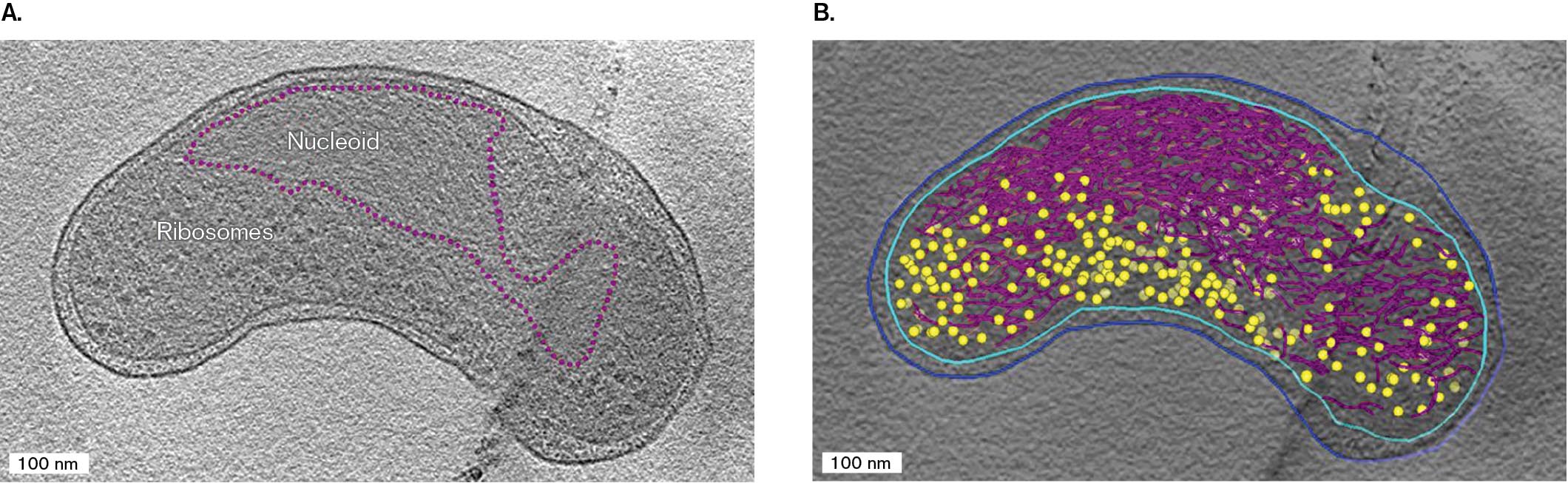
The cryo-EM micrograph in Figure 2.41A shows Pelagibacter, an ultrasmall bacterium found throughout the open oceans. Pelagibacter is a heterotroph adapted to the lowest concentrations of nutrients. It is one of the world’s most abundant life forms, and one of the smallest free-living cells (about 0.01 cubic micrometer). Little is known about its means of survival, with its streamlined genome and cell structure. The cell section reveals in detail the form of its Gram-negative outer membrane (blue), inner membrane (cyan), and periplasmic space between (Fig. 2.41B). Within the cytoplasm, we can see the DNA strands of nucleoid (red) and individual ribosomes (yellow). As small as the cell is, we can see its distinctive asymmetry of shape, a curved cell with one end pinched. The function of the asymmetry is unknown.

More information

Two Cryo-electron tomographs of the marine bacterium Pelagibacter, with different labeling that shows nucleoid D N A, ribosomes, inner membrane, and outer membrane.

A Cryo-electron tomograph shows a bean-shaped cell of Pelagibacter with the nucleoid outlined. It looks like a thin loop. Several ribosomes are visible within the cell. The cell is about 700 nanometers long and 200 nanometers wide.

A Cryo-electron tomograph shows a bean-shaped cell of Pelagibacter with 3 D models of internal structures. Yellow dots, representing ribosomes, are present throughout the cell. Purple strands, representing nucleoid DNA, follow the rough outline of the nucleoid seen in the first tomograph. Two lines follow the border of the cell. The inner line is light blue and represents the inner membrane. The outer line is dark blue and represents the outer membrane. The cells is about 700 nanometers long and 200 nanometers wide.

Note: Pelagibacter ubique is the first of several cultured isolates of the “SAR11” cluster of bacteria, originally identified by analysis of DNA sequences of bacteria in the Sargasso Sea near Bermuda. The SAR11 cluster has since been expanded beyond genus to the rank of order: Pelagibacterales, phylum Alphaproteobacteria.

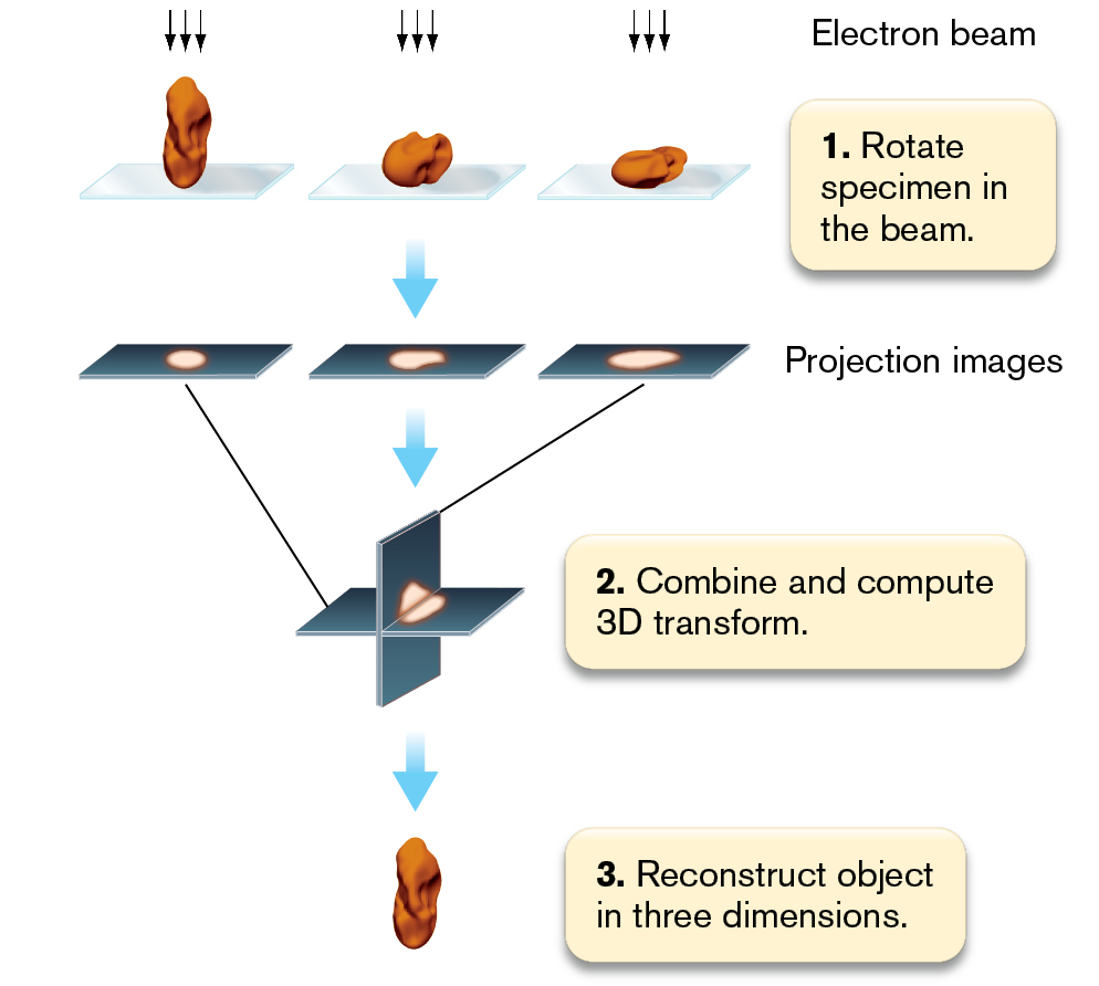
Tomography. Another innovation made possible by cryo-EM is tomography, the acquisition of projected images from different angles of a transparent specimen. Cryo-electron tomography, or electron cryotomography, avoids the need to physically slice the sample for thin-section TEM. The images from tomography are combined digitally to visualize objects in 3D, such as the Pelagibacter nucleoid and ribosomes (Fig. 2.41B). Repeated scans can be summed computationally to obtain an image at high resolution (Fig. 2.42). The scans are taken either at different angles or within different focal planes. Each different scan images a slightly different part of the cell. The summed scans then generate a 3D model.

More information

An illustration shows the construction of 3 D images in cryo-electron tomography. An irregularly shaped specimen is shown at 3 angles. At each angle, electron beams are directed down at the specimen. The corresponding text reads 1. Rotate Specimen in the beam. Next, three projection images show the shadow of the specimen angles. Next, a three dimensional plane combines the projection images. The corresponding text reads 2. Combine and compute 3 D transform. Finally, the reconstructed image of the Specimen is shown at the bottom. The corresponding text reads 3. Reconstruct object in three dimensions.

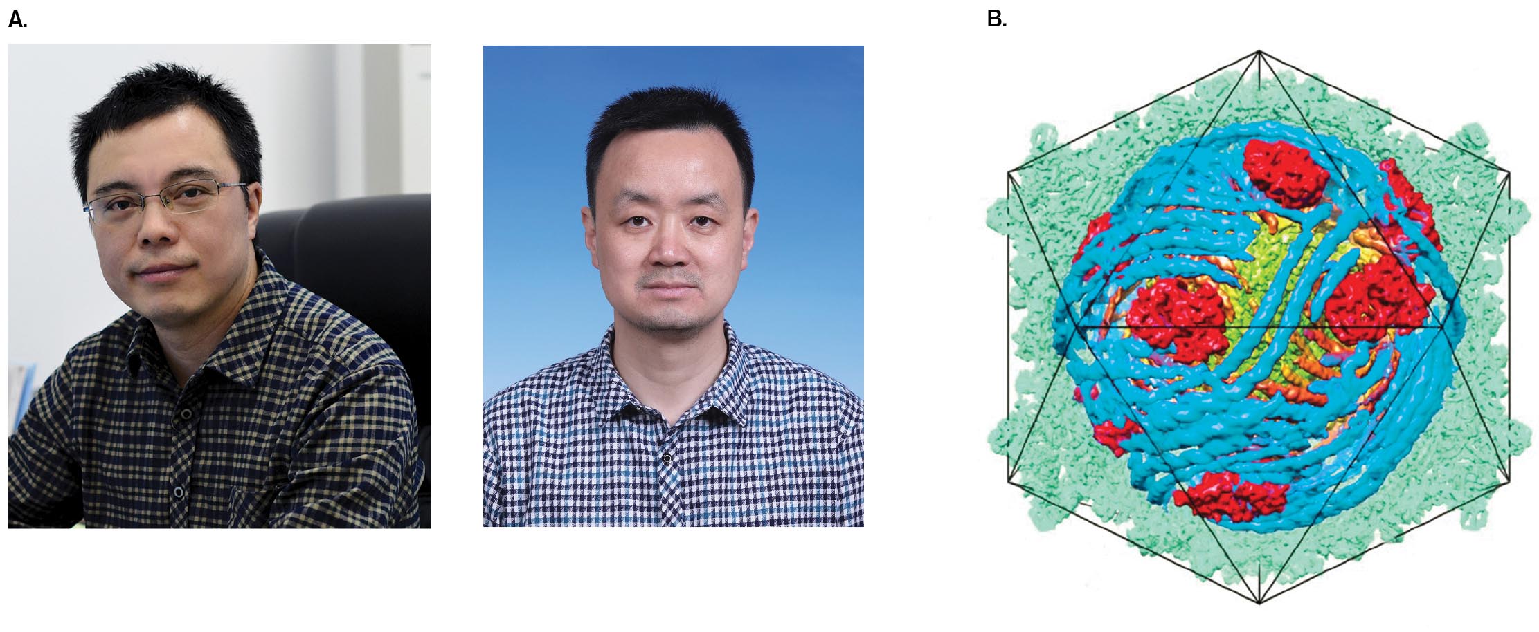
Modeling cell parts. One use of cryo-electron tomography is to generate high-resolution models of complex particles, such as viruses. For a symmetrical virus, particle images can be rotated for averaging. In addition, images of multiple particles can be averaged together. The digitally combined images can achieve high resolution, nearly comparable to that of X-ray crystallography. Chinese microscopists Hongrong Liu, at Hunan Normal University, and Lingpeng Cheng, at Tsinghua University, used cryo-EM to model cypovirus, a virus that infects silkworms and butterfly larvae (Fig. 2.43). Other viruses modeled recently include herpesvirus and human immunodeficiency virus (HIV) (presented in Chapter 11). Cryo-EM is especially useful for particles that cannot be crystallized for X-ray diffraction analysis, the most common means of molecular visualization.

More information

Photos of Hongrong Liu and Lingpeng Cheng are shown next to a Cypovirus model.

A photo of Hongrong Liu.

A photo of Lingpeng Cheng.

A model of the structure of Cypovirus. The model shows the virus structure of the capsid in which a group of red-colored R N A polymerase and blue colored R N A genome are packed inside the capsid.

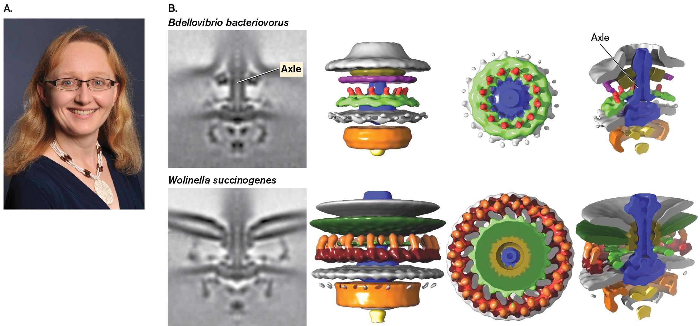
Another example is the modeling of rotary flagellar motors. Bonnie Chaban (Fig. 2.44A) and co-workers at Imperial College London used cryo-EM digital combination to obtain detailed models of the motors of Campylobacterales, a clade of bacteria including enteric pathogens. The models allowed reconstruction of each motor interior, including each axle (shown as violet). It was possible to compare the motors from related bacteria, such as the Escherichia coli predator Bdellovibrio and the rumen symbiont Wolinella (Fig. 2.44B). The comparison enabled computation of a phylogenetic tree of motor evolution—something once thought impossible because of the precision requirements of a rotary device.

More information

A photo of Bonnie Chaban and two Cryo-electron tomographs of motors of bacterial flagella with accompanying 3 D models.

A photo of Bonnie Chaban.

Two Cryo-electron tomographs of motors of bacterial flagella with accompanying 3 D models. The first tomograph shows the structure of the axle in Bdellovibrio bacteriovorus. It looks like a vertical tube with structures on the top and bottom. To the right shows the models of gear, wheel, and axle. Different ring shaped layers surround a central column. The second tomograph shows the structure of a motor with two flagella in Wolinella succinogenes. It looks like a vertical tube with structures on the top and bottom as well as long projections coming off the top. To the right shows the models of bearing, wheel, and axle. Different ring shaped layers surround a central column.

Model of a cell. Cryo-EM models of a motor are impressive, but can we build a 3D model of an entire cell? Grant Jensen and colleagues at the California Institute of Technology use cryo-electron tomography to visualize an entire flash-frozen bacterium. Such a model includes all the cell’s parts and their cytoplasmic connections—and reveals new structures never seen before.

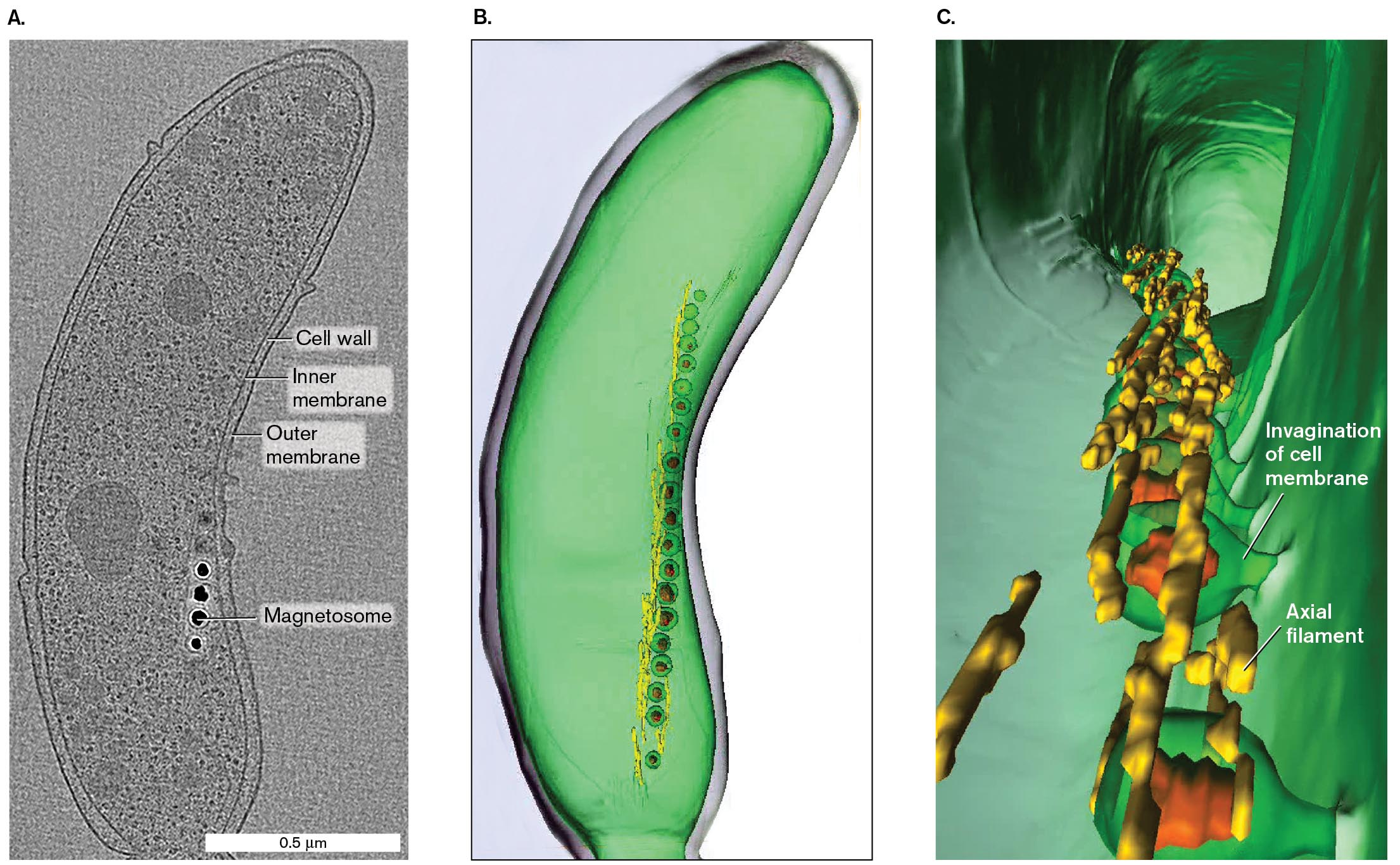
The cell modeled in Figure 2.45 is Magnetospirillum magneticum, a bacterium that can swim along Earth’s magnetic field in order to reach deeper, low-oxygen water. To orient along magnetic field lines, the cell contains a string of magnetic particles composed of the mineral magnetite (iron oxide; Fe₃O₄). A cryo-EM section through the bacterium (Fig. 2.45A) shows fine details, including the inner membrane (equivalent to the cell membrane), peptidoglycan cell wall, and outer membrane, an outer covering found in Gram-negative bacteria. Four dark magnetosomes (particles of magnetite) appear in a chain, each surrounded by a vesicle of membrane. How do cells form such intracellular structures? For some clues, see eResearch Activity 2.

Figure 2.45B models the magnetosomes, reconstructed using multiple cryo-EM scans across the volume of the cell. The magnetosomes are colorized red, each surrounded by a membrane vesicle (green). The vesicles are organized within the cell by a series of protein axial filaments, colorized yellow. Figure 2.45C shows an expanded image of the magnetosomes viewed from the cell interior. This expansion reveals that the magnetosome vesicles consist of invaginations from the cell membrane. Thus, the 3D model shows how the magnetite particles are fixed in position by invaginated membranes and held in a line by axial filaments.

More information

Three images show increasing detail of the structure of Magnetospirillum magneticum based on cryo-electron tomography.

A cryo-electron tomograph shows the labeled structure of Magnetospirillum magneticum. The labeled parts are cell wall, inner membrane, outer membrane, and the four dots near to the inner membrane are labeled as magnetosomes. The cell is a bean shaped structure of about 1.5 micrometers in length and 0.5 micrometer in width.

A 3 D structure of M. magneticum with several magnetosomes. It is green and bean shapes. The magnetosomes form a vertical chain inside on one side.

A 3 D model of the cell interior of M. magneticum. The internal structure appears as a hollow tunnel with several magnetosomes embedded in the cell membrane. The point where the magnetosomes embed in the cell membrane is labeled, invagination of cell membrane. Axial filaments are identified between magnetosomes.

Scanning Probe Microscopy

Scanning probe microscopy (SPM) enables nanoscale observation of cell surfaces. Unlike electron microscopy, some forms of SPM can be used to observe live bacteria in water or exposed to air.

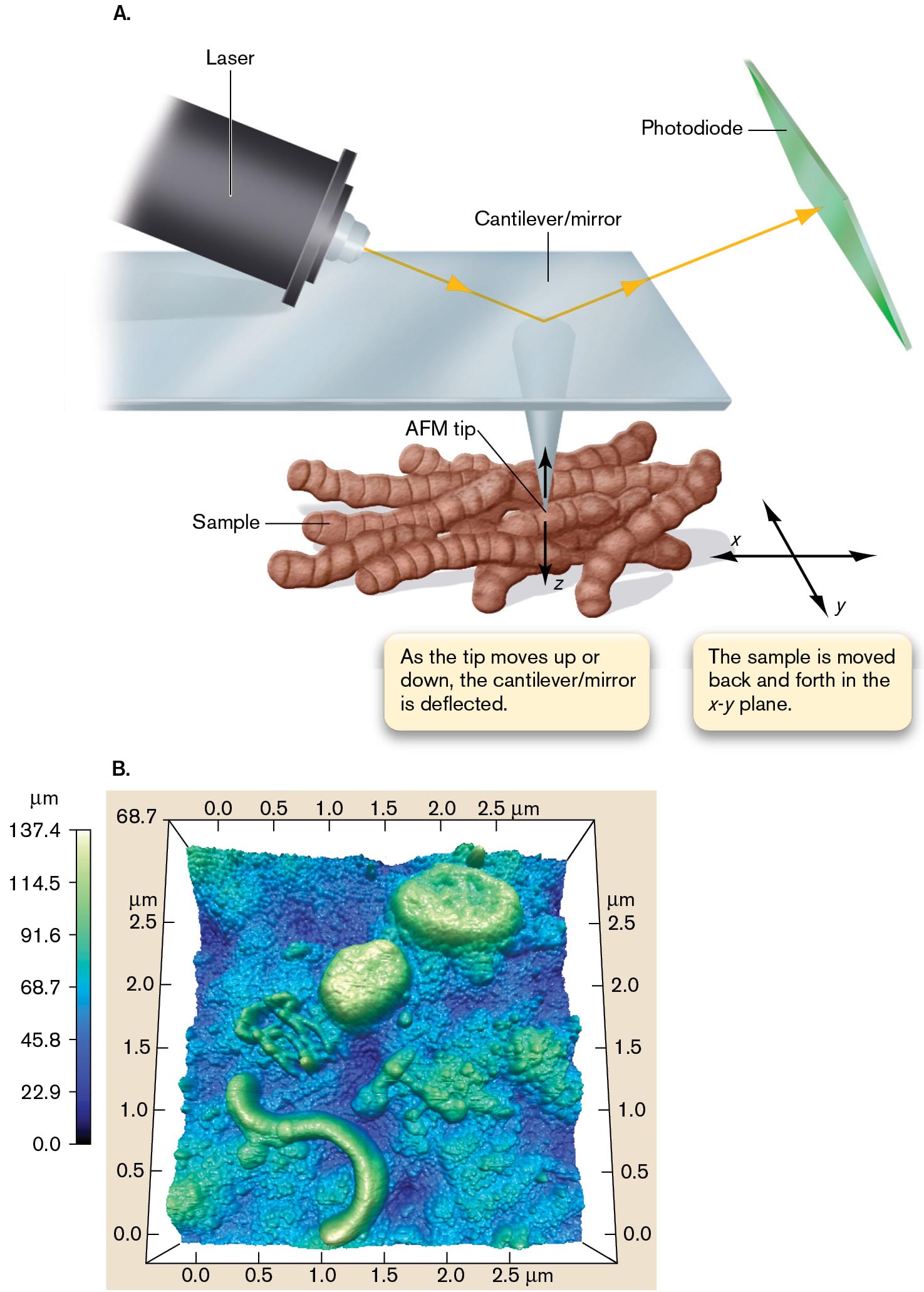
SPM techniques measure a physical interaction, such as the “atomic force” between the sample and a sharp tip. Atomic force microscopy (AFM) measures the van der Waals forces between the electron shells of adjacent atoms of the cell surface and the sharp tip. In AFM, an instrument probes the surface of a sample with a sharp tip a couple of micrometers long and often less than 10 nm in diameter (Fig. 2.46A). The tip is located at the free end of a lever that is 100–200 µm long. The lever is deflected by the force between the tip and the sample surface. Deflection of the lever is measured by a laser beam reflected off a cantilever attached to the tip as the sample scans across. The measured deflections allow a computer to map the topography of cells in liquid medium and at a resolution below 1 nm.

In Figure 2.46B, AFM was used to observe live bacteria collected on a filter, from seawater off the coast of California. Two round bacteria and a helical bacterium can be seen (raised regions, green-white). The cells were observed in water suspension, without stain. Thus, AFM can help assess the ecological contributions of marine bacteria that cannot be cultured.

More information

An illustration and a graph show the visualization of untreated cells enabled by atomic force microscopy.

An illustration shows the basic structure of the atomic force microscope. A horizontal plane labeled cantilever or mirror has an atomic force microscope tip pointed at a group of rod-shaped cells labeled as a sample at the bottom. As the tip moves up or down, the cantilever or mirror is deflected. This measures the sample on the z-axis. A note reads, the sample is moved back and forth in the x y plane. A laser emits a beam down diagonally towards the top of the A F M tip, and the light changes direction to move upward to hit the plane at the top right labeled as a photodiode.

An A F M image of live bacteria with scales in the X, Y, and Z axis. The image is a square. Each side of the image has a scale ranging from 0.0 to 2.5 micrometers in increments of 0.5 micrometer. The image is colorized. A color scale adjacent to the image ranges from 0.0 to 137.4 micrometers in increments of 22.9 micrometers. At a height of 137.4 micrometers, the color is light green. At a height of 0.0 micrometer, the color is dark blue. Several different bacteria are visible in the image, with varying heights, lengths, and widths.

Thought Question

2.9 How could you use atomic force microscopy to study the effect of an antibiotic on Pseudomonas aeruginosa contamination of medical catheters?

ANSWER ANSWER

Bacteria colonize catheters by forming a biofilm, a structure of cells that grow attached to each other and to the substrate. The height and volume of a biofilm can be measured by AFM. As shown in Figure 2.46, deflection of the tip of the cantilever indicates very precise measurements of thickness of a biofilm, allowing three-dimensional mapping. An antibiotic can be added at various concentrations, and the height and volume of the biofilm can be measured over time. This procedure will indicate how an antibiotic affects biofilm formation on a catheter.

X-Ray Diffraction Analysis

To know a cell, we need to isolate the cell’s individual molecules. The major tool used at present to visualize a molecule is X-ray diffraction analysis, or X-ray crystallography. Much of our knowledge of microbial genetics (see Chapters 7–12) and metabolism (see Chapters 13–16) comes from crystal structures of key macromolecules.

Unlike microscopy, X-ray diffraction does not present a direct view of a sample, but instead generates computational models. Dramatic as the models are, they can only represent particular aspects of electron clouds and electron density that are fundamentally “unseeable.” That is why we represent molecular structures in different ways that depend on the context—by electron density maps, as models defined by van der Waals radii, or as stick models. Proteins are frequently presented in a cartoon form that shows alpha helix and beta sheet secondary structures.

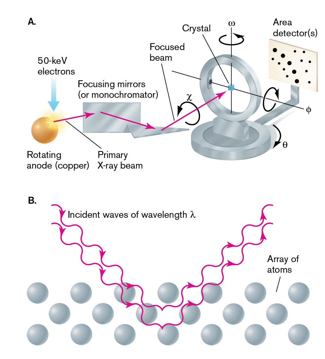
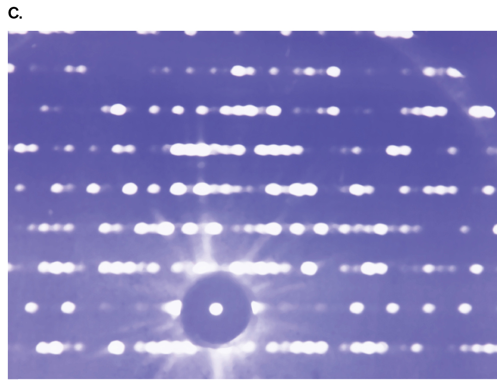
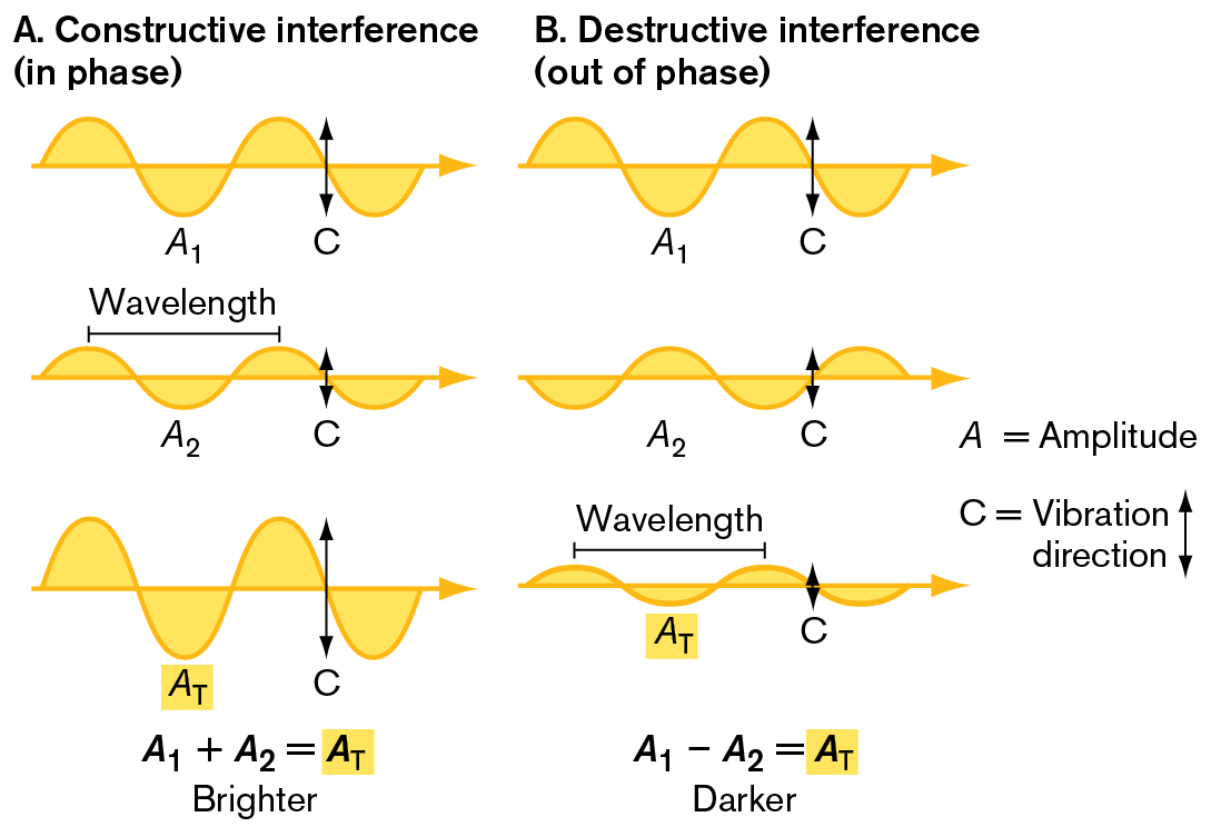
For a molecule that can be crystallized, X-ray diffraction makes it possible to fix the position of each individual atom in the molecule. Atomic resolution is possible because the wavelengths of X-rays are much shorter than the wavelengths of visible light and are comparable to the size of atoms. X-ray diffraction is based on the principle of wave interference (see Fig. 2.19). The interference pattern is generated when a crystal containing many copies of an isolated molecule is bombarded by a beam of X-rays (Fig. 2.47A). The wavefronts associated with the X-rays are diffracted as they pass through the crystal, causing interference patterns. In the crystal, the diffraction pattern is generated by a symmetrical array of many sample molecules (Fig. 2.47B). The more copies of the molecule in the array, the narrower the interference pattern and the greater the resolution of atoms within the molecule. Diffraction patterns obtained from the passage of X-rays through a crystal (Fig. 2.47C) can be analyzed by computation to develop a precise structural model for the molecule, detailing the position of every atom in the structure.

More information

Two illustrations of x-ray crystallography and the diffraction pattern from a crystal are shown.

An illustration depicts x-ray crystallography. The apparatus consists of a sphere labeled as rotating anode, or copper, focusing mirrors, or monochromators, a focused beam, a crystal placed in the center of the circular coil, and a plane with several dots labeled as area detectors. A horizontal line inside the circular coil is labeled as theta with rotation and the vertical line with omega rotation. 50 Kilo electron volt electrons enter into the rotating anode. An arrow labeled primary x-ray beam points from the anode to the focusing mirrors and enters into the focused beam at chi rotation and leads to the crystal. This produces a pattern on the area detectors.

An illustration shows incident waves moving through an array of atoms. The waves have a wavelength of lambda and follow a V shape as the enter and then exit the atom array.

More information

X-ray crystallography shows several bonded crystals arranged in multiple rows in the diffraction pattern. They look like rows of dots with some of the dots close enough that they blur together.

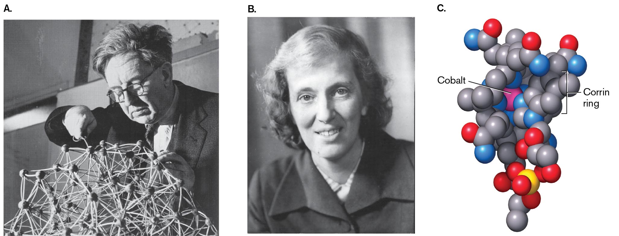
The application of X-ray crystallography to complex biological molecules was pioneered by the Irish crystallographer John Bernal (1901–1971; Fig. 2.48A). Bernal was particularly supportive of women students and colleagues, including Rosalind Franklin (1920–1958), who made important discoveries about DNA and RNA, and Nobel laureate Dorothy Crowfoot Hodgkin (1910–1994). Hodgkin (Fig. 2.48B) solved the crystal structures of penicillin and vitamin B₁₂ (Fig. 2.48C), as well as one of the first protein structures—that of the hormone insulin.

More information

Two photos of John Bernal and Dorothy Hodgkin are shown next to a space filling model of Vitamin B subscript 12.

A photo of John Bernal working on a complex ball and stick molecular model.

A photo of Dorothy Hodgkin.

A space filling model of Vitamin B subscript 12. It consists of a space-filling model of a pink atom, labeled Cobalt, in the center. It is bonded with several spheres of different colors. A part closer to the cobalt atom is labeled as, corrin ring.

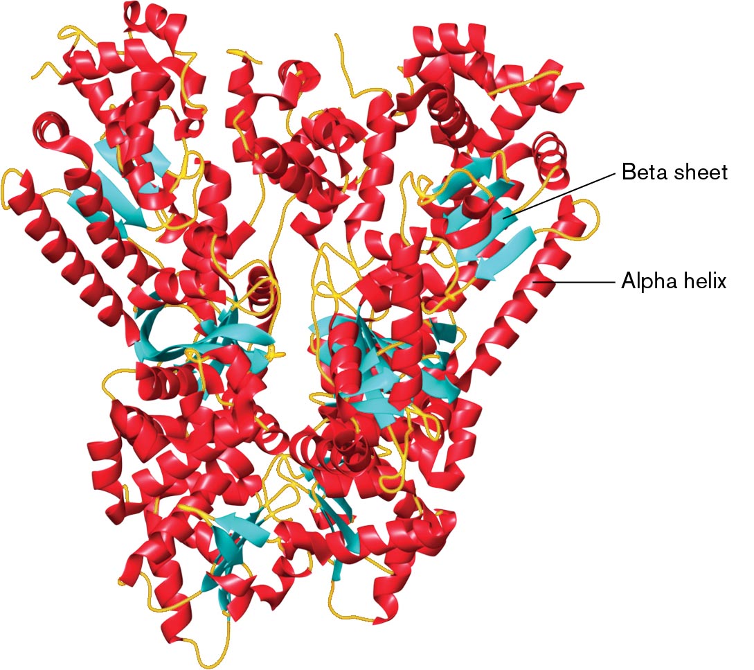
Today, X-ray data undergo digital analysis to generate sophisticated molecular models, such as the one seen in Figure 2.49 of anthrax lethal factor, a toxin produced by Bacillus anthracis that kills the infected host cells. The model for anthrax lethal factor was encoded in a Protein Data Bank (PDB) text file that specifies coordinates for all atoms of the structure. The Protein Data Bank is a worldwide database of solved X-ray structures, freely available on the Internet. Visualization software is used to present the structure as a “ribbon” of amino acid residues, color-coded for secondary structure. The ribbon diagram method was developed by Jane S. Richardson and is also known as the “Richardson diagram.” In Figure 2.49, the red coils represent alpha helix structures, whereas the blue arrows represent beta sheets (for a review of protein structures, see eAppendix 1).

More information

A three dimensional model of the protein structure of anthrax lethal factor. It is bonded with thick arrows labeled as a beta-sheet and spiral-shaped structures labeled as an alpha helix. The majority of the structure is made of alpha helices. There are two denser lobes next to each other that form a shape somewhat like butterfly wings.

Note: Molecular and cellular biology increasingly rely on visualization in 3D. Many of the molecules illustrated in this book are based on structural models deposited in the Protein Data Bank, as indicated by the PDB file code. Each PDB file can be viewed in 3D in the browser.

A limitation of X-ray analysis is the unavoidable deterioration of the specimen under bombardment by X-rays. The earliest X-ray diffraction models of molecular complexes such as the ribosome relied heavily on components from thermophilic bacteria and archaea that grow at high temperatures. Because thermophiles have evolved to grow under higher thermal stress, their macromolecular complexes are often more stable and therefore easier to crystallize than homologous proteins from organisms that grow at moderate temperatures.

X-ray diffraction analysis of crystals from a wide range of sources was made possible by cryocrystallography. In cryocrystallography, as in cryo-EM, crystals are frozen rapidly to liquid-nitrogen temperature. The frozen crystals have greatly decreased thermal vibrations and diffusion, thus lessening the radiation damage to the molecules. Models based on cryocrystallography can present multisubunit structures such as the bacterial ribosome complexed with transfer RNAs and messenger RNA (presented in Chapter 8).