1.10 Summary
New Concepts
Atomic orbitals (mathematically described by wave functions) are defined by four quantum numbers, n, l, ml, and s. Electrons may have only certain energies determined by these quantum numbers. Orbitals have different, well-defined shapes: s orbitals are spherically symmetric, p orbitals are roughly dumbbell shaped, and d and f orbitals are more complicated. An orbital may contain a maximum of two electrons.
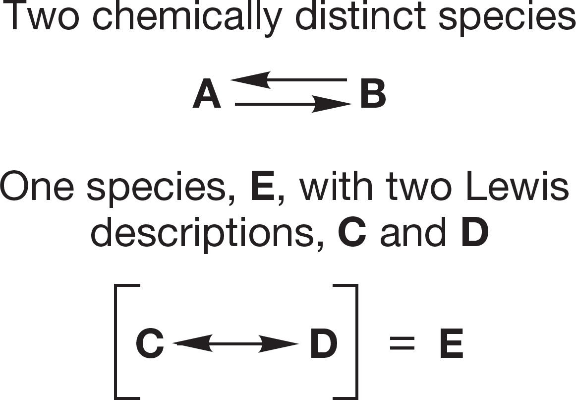
Some molecules cannot be well described by a single Lewis structure but are better represented by two or more different electronic descriptions. This phenomenon is called resonance. Be sure you are clear on the difference between an equilibrium between two different molecules and the description of a single molecule using several different resonance forms.
When two orbitals overlap, two new orbitals are formed: one is lower in energy than the starting orbitals, and the other is higher in energy than the starting orbitals. Electrons placed in the new, lower-energy orbital are stabilized because their energy is lowered. The overlap of atomic orbitals to form molecular orbitals and the attendant stabilization of electrons as they move from the atomic orbitals to the lower-energy molecular orbitals are the basis of covalent bonding.
This orbital-forming process can be generalized: When you mix n orbitals into the calculation, the mathematical solution will produce n new orbitals.
Key Terms
anion
antibonding molecular orbital
arrow formalism, curved arrow formalism, or electron pushing
atom
atomic orbital
aufbau principle
bond dissociation energy (BDE)
bonding molecular orbital
cation
covalent bond
delocalization
dipole moment
electron
electron affinity
electronegativity
electrophile
endothermic reaction
enthalpy change (ΔH°)
exothermic reaction
formal charge
functional group
Heisenberg uncertainty principle
heterolytic bond cleavage
homolytic bond cleavage
Hund’s rule
ion
ionic bond
ionization potential
Lewis acid
Lewis base
Lewis structure
lone-pair electrons
molecular orbital
node
nonbonding electrons
nonbonding orbital
nucleophile
nucleus
octet rule
orbital
orbital interaction diagram
orthogonal orbitals
paired spin
parallel spin
Pauli principle
polar covalent bond
quantum numbers
resonance arrow
resonance forms
unpaired spin
valence electrons
wave function (ψ)
weighting factor
Reactions, Mechanisms, and Tools
There are no reactions to speak of yet, but we have developed a few tools in this first chapter.
We draw Lewis structures by representing each valence electron by a dot. These dots are transformed into vertical arrows if it is necessary to show electron spin. Exceptions are the ls electrons, which are held too tightly to be significantly involved in bonding except in hydrogen. These electrons are not shown in Lewis structures except in H and He. Somewhat more abstract representations of molecules are made by showing electron pairs in bonding orbitals as lines—the familiar bonds between atoms.
The double-headed resonance arrow is introduced to cope with those molecules that cannot be adequately represented by a single Lewis structure. Different electronic representations, called resonance forms, are written for the molecule. The molecule is better represented by a combination of all the resonance forms. Be very careful to distinguish the resonance phenomenon from chemical equilibrium. Resonance forms give multiple descriptions of a single species. Equilibrium describes two (or more) different molecules.
The curved arrow formalism is introduced to show the flow of electrons. This critically important device is used both in drawing resonance forms and in sketching electron flow in reactions throughout this book.
The formation of a bonding molecular orbital (lower in energy) and an antibonding molecular orbital (higher in energy) from the overlap of two atomic orbitals can be shown in an orbital interaction diagram (Fig. 1.50). Electrons are represented by vertical arrows that indicate electron spin (↑ or ↓). Remember that only two electrons can be stabilized in the bonding orbital and that two electrons in the same orbital must have opposite spins.
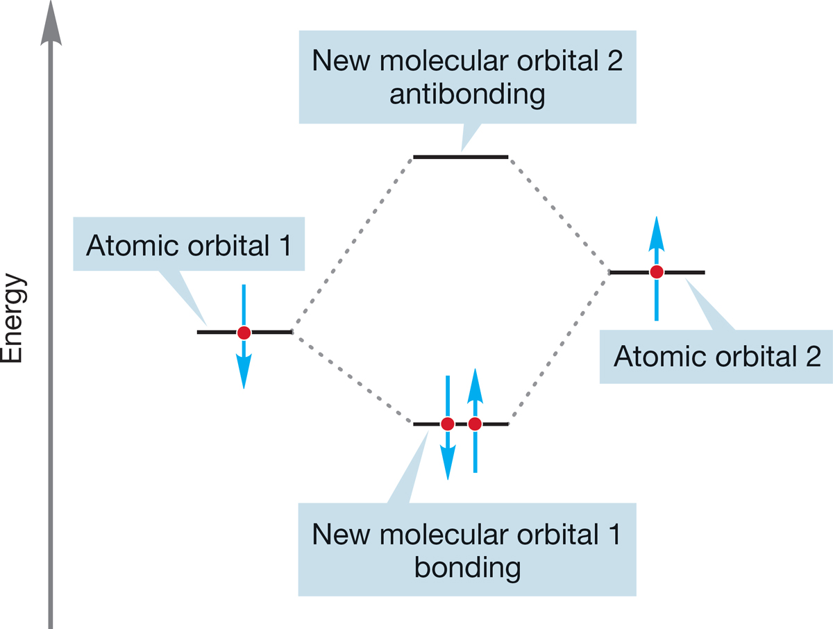
FIGURE 1.50 The overlap of two atomic orbitals produces two new molecular orbitals.
Common Errors
Here, and in similar sections throughout the book, we will take stock of some typical errors made by those who attempt to come to grips with organic chemistry.
Electrons are not baseballs. Nothing is harder for most students to grasp than the consequences of this observation. Electrons behave in ways that the moving objects in our ordinary lives do not. No one who has ever kicked a soccer ball or caught a fly ball can doubt that on a practical level, it is possible to determine both the position and speed of such an object at the same time. However, Heisenberg demonstrated that this is not true for an electron. We cannot know both the position and speed of an electron at the same time.
Baseballs move at a variety of speeds (energies), and a baseball’s energy depends only on how hard we throw it. Electrons are restricted to certain energies (orbitals) determined by the values of quantum numbers. Electrons behave in other strange and counterintuitive ways. For example, we have seen that a node is a region of space of zero electron density. Yet, an electron occupies an entire 2p orbital in which the two halves are separated by a nodal plane. A favorite question, How does the electron move from one lobe of the orbital to the other? simply has no meaning. The electron is not restricted to one lobe or the other but occupies the whole orbital (Fig. 1.51). Mathematics makes these properties seem inevitable; intuition, derived from our experience in the macroscopic world, makes them very strange.
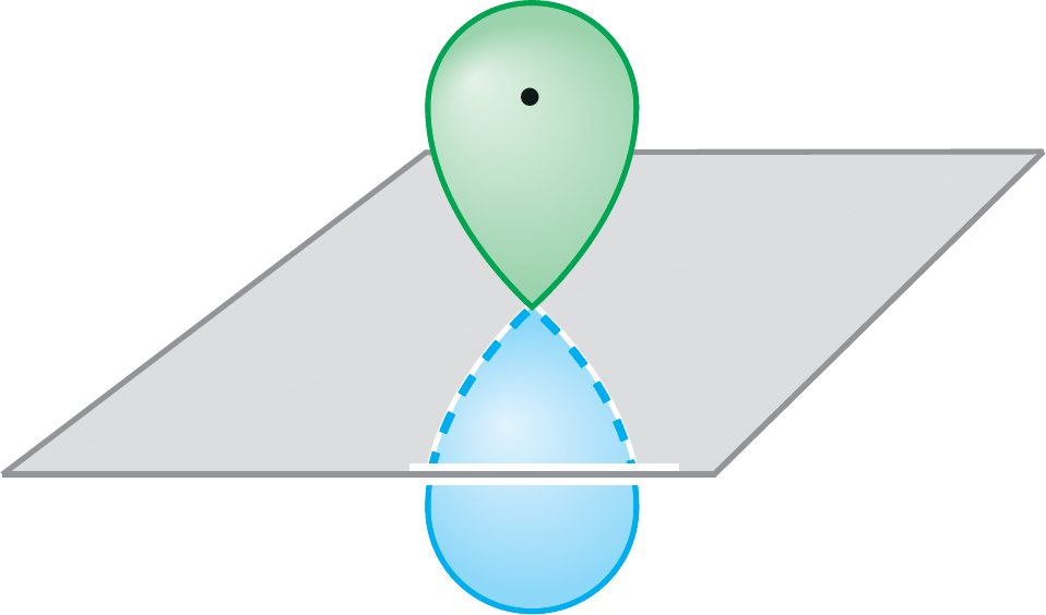
FIGURE 1.51 An electron occupies an entire 2p (or other) orbital—it is not restricted to only one lobe.
It is easy to confuse resonance with equilibrium. On a mundane, but nonetheless important level, this confusion appears as a misuse of the arrow convention. Two arrows separate two entirely different molecules (A and B), each of which might be described by several resonance forms. The amount of A and B present at equilibrium depends on the equilibrium constant. The double-headed resonance arrow separates two different electronic descriptions (C and D) of the same species, E (see Fig. 1.31).
Construction of molecular orbitals through combinations of atomic orbitals (or other molecular orbitals) can be daunting, at least in the beginning. Remember these hints:
1. The number of orbitals produced at the end must equal the number at the beginning. If you start with n orbitals, you must produce n new orbitals. This is a way to check your work as it proceeds.
2. Keep the process as simple as you can. Use what you know already, and combine orbitals in as symmetrical a fashion as you can.
3. The closer in energy two orbitals are, the more strongly they interact. At this level of theory, you need only interact the pairs of orbitals closest in energy to each other.
4. The more in-phase (+/+ or −/−) overlap there is between mixing orbitals, the lower is the energy of the new bonding orbital. Out-of-phase overlap (+/−) leads to a new orbital of higher energy. Electrons in low-energy orbitals are more stable than electrons in higher-energy orbitals.
5. When orbitals interact in a bonding way (same sign of the wave function), the energy of the resulting orbital is lowered; when they interact in an antibonding way (different signs of the wave function), the energy of the resulting orbital is raised.
6. When two orbitals interact, the only options for mixing are adding (in-phase mixing) or subtracting (out-of-phase mixing). When three orbitals interact, there will be three ways to mix the orbitals. With four orbitals there are four possible combinations, and so on.
7. To order the orbitals in energy, count the nodes. For a given molecule, the more nodes in an orbital, the higher it is in energy.
These methods will become much easier than they seem at first, and they will provide a remarkable number of insights into structure and reactivity not easily available in other ways.
The sign convention for exothermic and endothermic reactions seems to be a perennial problem. In an exothermic reaction, the products are more stable than the starting materials. Heat is given off in the reaction, and ΔH° is given a minus sign. Thus, for the reaction A + B → C, ΔH° = −x kcal/mol. An endothermic reaction is just the opposite. Energy must be applied to form the less stable products from the more stable starting material. The sign convention gives ΔH° a plus sign. Thus, A + B → C, ΔH° = +x kcal/mol.