1.2 Atoms and Atomic Orbitals
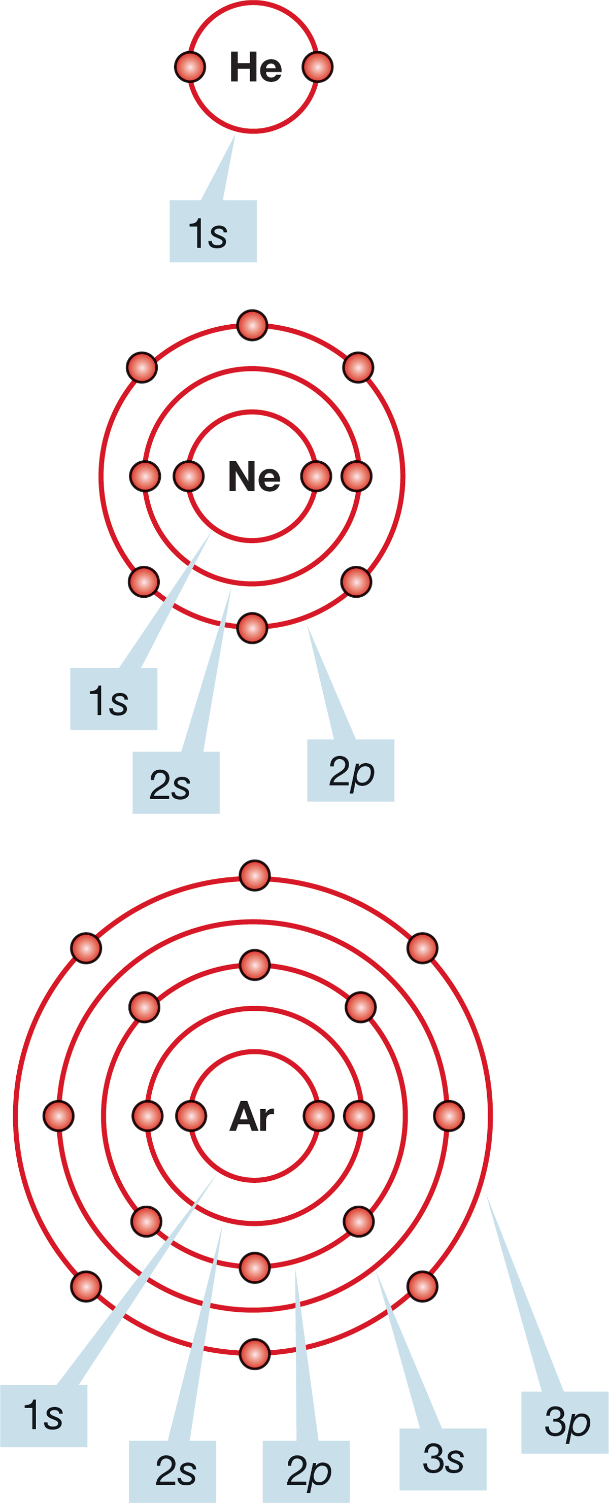
FIGURE 1.1 Schematic representations of He, Ne, and Ar.
In a neutral atom, the nucleus, or core of positively charged protons and neutral neutrons, is surrounded by a number of negatively charged electrons equal to the number of protons. If the number of electrons and protons is not equal, the atom must be charged and is called an ion. A negatively charged atom or molecule is called an anion; a positively charged species is a cation. (One of the tests of whether or not you know how to “talk organic chemistry” is the pronunciation of the word cation. It is kat-eye-on, not kay-shun.)
The energy required to remove an electron from an atom to form a cation is called the ionization potential. In general, the farther away an electron is from the nucleus, the easier it is to remove the electron, and thus the ionization potential is lower.
Much of the chemistry of atoms is dominated by the gaining or losing of electrons to achieve the electronic configuration of one of the noble gases (He, Ne, Ar, Kr, Xe, and Rn). The noble gases have especially stable filled shells of electrons: 2 for He, 10 for Ne (2 + 8), 18 for Ar (2 + 8 + 8), and so on. The idea that filling certain shells creates especially stable configurations is known as the octet rule. With the exception of the first shell, called the 1s orbital, which can hold only two electrons, all shells fill with eight electrons; thus, this rule specifies an octet. The second shell can hold eight electrons: two in the subshell called the 2s orbital and six in the subshell 2p orbitals. We will soon explain these numbers and names, but first we need to understand the labels. Figure 1.1 shows schematic illustrations of three noble gases and their orbital designations. These pictures do not give good three-dimensional representations of these species, but they do show subshell occupancy. Better pictures are forthcoming.
The two electrons surrounding the helium (He) nucleus completely fill the first shell, and for this reason it is most difficult to remove an electron from He. Helium has an especially high ionization potential, 24.6 eV/atom = 566 kcal/mol = 2370 kJ/mol.5 Likewise, the chemical inertness of the other noble gases, which also have high ionization potentials, is the result of the stability of their filled valence shells.
Electrons can be added to atoms as well as removed. The energy that is released by adding an electron to an atom to form an anion is called the atom’s electron affinity, which is measured in electron volts. The noble gases have very low electron affinities. Conversely, atoms to which addition of an electron would complete a noble gas configuration have high electron affinities. The classic example is fluorine: The addition of a single electron yields a fluoride ion, F−, which has the electronic configuration of Ne. Both F− and Ne are 10-electron species, as Figure 1.2 shows.
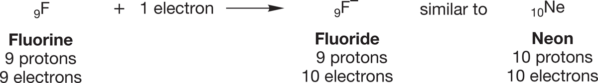
FIGURE 1.2 Addition of an electron to a fluorine atom gives a fluoride ion.
HELIUM
Helium (He) is the only substance that remains liquid under its own pressure at the lowest temperature recorded. Helium is present at only ~5 ppm in Earth’s atmosphere, but it reaches substantially higher concentrations in natural gas, from which it is obtained. Helium is formed from the radioactive decay of heavy elements. For example, a kilogram of uranium gives 865 L of helium after complete decay. There’s not much helium on Earth, but there is a lot in the universe. About 23% of the known mass of the universe is helium, mostly produced by thermonuclear fusion reactions between hydrogen nuclei in stars. So, an outside observer of our universe (whatever that means!) would probably conclude that helium is some of the most important stuff around.
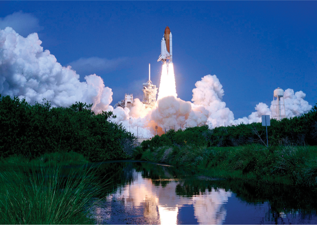
The NASA space shuttle launched on July 8, 2011, used more than 28,000 L of liquid helium. The transition from liquid to gaseous helium provided necessary pressure to the system, and the helium helped push out the combustion products formed during the liftoff.
CONVENTION ALERT
Atomic Numbers of Elements
Single atoms, such as the fluorine atom shown on the left in Figure 1.2, are often written in the form  , where W represents the mass number (number of protons and neutrons in the nucleus), Z represents the atomic number (number of protons in the nucleus), and C is the element symbol, here C for carbon. Thus, this notation for fluorine is
  . In this book, the superscript W value is omitted, which leads to the 9F and 10Ne symbols you see in Figure 1.2.
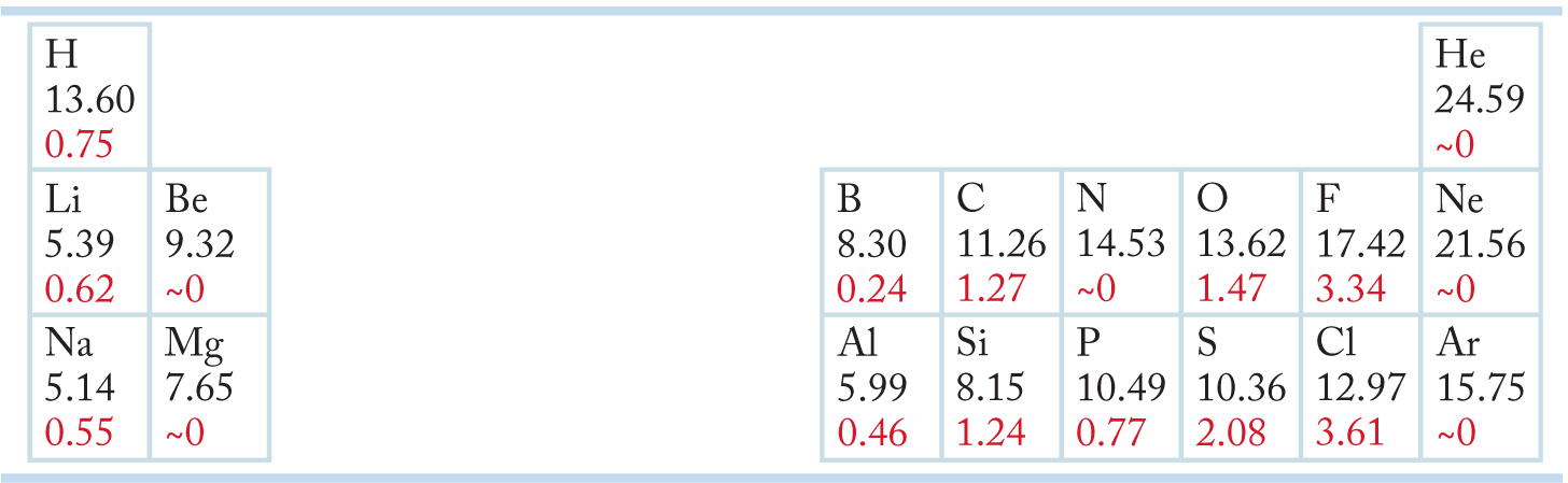
Table 1.1 shows ionization potentials and electron affinities of some elements arranged as in the periodic table. Notice that with the exception of hydrogen, atoms with low ionization potentials, which are atoms that have easily removed electrons, cluster on the left side of the periodic table, and atoms with high electron affinities, which are atoms that accept electrons easily, are on the right side (excluding the noble gases).
TABLE 1.1 Some Ionization Potentials (Black) and Electron Affinities (Red) in Electron Volts
Atoms having low ionization potentials often transfer an electron to atoms having high electron affinities, forming ionic bonds. In an ionically bonded species, such as sodium fluoride (Na+F−), the atoms are held together by the electrostatic attraction of the opposite charges. In sodium fluoride, both Na+ and F− have filled second shells, and each has achieved the stable electronic configuration of the noble gas Ne. In potassium chloride (K+Cl−), both ions have the electronic configuration of Ar, another noble gas (Fig. 1.3).

FIGURE 1.3 In the ionic compounds NaF and KCl, each atom can achieve a noble gas electronic configuration with a filled octet of electrons.
Ionically bonded compounds are traditionally the province of inorganic chemistry. Nearly all of the compounds of organic chemistry are bound not by ionic bonds but rather by covalent bonds, which are bonds formed by the sharing of electrons.
1.2a Quantum Numbers We have just developed pictures of some atoms and ions. Let’s elaborate a bit to provide a fuller picture of atomic orbitals. Your reward for bearing with an increase in complexity will be a much-increased ability to think about structure and reactivity. The most useful models for explaining and predicting chemical behavior focus on the qualitative aspects of atomic (and molecular) orbitals, so it is time to learn more about them.
The electrons in atoms do not occupy simple circular orbits. To describe an electron in the vicinity of a nucleus, Erwin Schrödinger (1887–1961) developed a formula called a wave equation. Schrödinger recognized that electrons have properties of both particles and waves. The solutions to Schrödinger’s wave equation, called wave functions and written Ψ (pronounced “sigh”), have many of the properties of waves. They can be positive in one region, negative in another, or zero in between.
An orbital is mathematically described by a wave function, ψ, and the square of the wave function, ψ2, is proportional to the probability of finding an electron in a given volume. There are regions or points in space where ψ and ψ2 are both 0 (zero probability of finding an electron in these regions), and such regions or points are called nodes. However, ψ2 does not vanish at a large distance from the nucleus but rather maintains a finite value, even if inconsequentially small.
Each electron is described by a set of four quantum numbers. Quantum numbers are represented by the symbols n, l, ml, and s. The first two quantum numbers define the orbital of the electron. The first one, called the principal quantum number, is represented by n and may have the integer values n = 1, 2, 3, 4, and so on. It is related to the distance of the electron from the nucleus and hence to the energy of the electron. It describes the atomic shell the electron occupies. The higher the value of n, the greater the average distance of the electron from the nucleus and the greater the electron’s energy. The principal quantum number of the highest-energy electron of an atom also determines the row occupied by the atom in the periodic table. For example, the electron in H and the two electrons in He are all n = 1, as Table 1.2 shows, and so these two atoms are in the first row of the table. The principal quantum number in Li, Be, B, C, N, O, F, and Ne is n = 2, which tells us that electrons can be in the second shell for these atoms and places the atoms in the second row. The elements Na, Mg, Al, Si, P, S, Cl, and Ar are in the third row, and orbitals for the electrons in these atoms correspond to n = 1, 2, or 3.
TABLE 1.2 Principal Quantum Number (n) of the Highest-Energy Electron
Atom |
n |
H, He |
1 |
Li, Be, B, C, N, O, F, Ne |
2 |
Na, Mg, Al, Si, P, S, Cl, Ar |
3 |
The second quantum number, l, is related to the shape of the orbital and depends on the value of n. It may have only the integer values l = 0, 1, 2, 3, . . . , (n − 1). So, for an orbital for which n = l, l must be 0; for n = 2, l can be 0 or 1; and for n = 3, the three possible values of l are 0, 1, and 2.
Each value of l signifies a different orbital shape. We shall learn about these shapes in a moment, but for now just remember that each shape is represented by a letter. The orbital for which l = 0 is spherical, and the letter s is used to designate all spherical orbitals. For higher values of l, we do not have the convenience of easily remembered letters the way we do with “s for spherical.” Instead, you just have to remember that p is used for orbitals for which l = 1, d is used for those for which l = 2, and f is used for l = 3. These letters associated with the various values of l lead to the common orbital designations shown in Table 1.3.
TABLE 1.3 Relationship between n and l
n |
l |
Orbital Designation |
1 | 0 | 1s |
2 | 0 | 2s |
2 | 1 | 2p |
3 | 0 | 3s |
3 | 1 | 3p |
3 |
2 |
3d |
The third quantum number, ml, depends on l. It may have the integer values −l, . . . , 0, . . . , +l, and is related to the orientation of the orbital in space. Table 1.4 presents the possible values of n, l, and ml for n = 1, 2, and 3. Orbitals of the same shell (n) and the same shape (l) are at the same energy regardless of the ml value.
TABLE 1.4 Relationship between n, l, and ml
n |
l |
ml |
Orbital Designation |
1 |
0 |
0 |
1s |
2 |
0 |
0 |
2s |
2 |
1 |
−1 |
2p |
2 |
1 |
0 |
2p |
2 |
1 |
+1 |
2p |
3 |
0 |
0 |
3s |
3 |
1 |
−1 |
3p |
3 |
1 |
0 |
3p |
3 |
1 |
+1 |
3p |
3 |
2 |
−2 |
3d |
3 |
2 |
−1 |
3d |
3 |
2 |
0 |
3d |
3 |
2 |
+1 |
3d |
3 |
2 |
+2 |
3d |
Finally, there is s, the spin quantum number, which may have only the two values ±1/2.
Table 1.5 lists all the possible combinations of quantum numbers through n = 3.
TABLE 1.5 Possible Combinations of Quantum Numbers for n = 1, 2, and 3
n |
l |
ml |
s |
Orbital Designation |
1 |
0 |
0 |
|
1s |
2 |
0 |
0 |
|
2s |
2 |
1 |
−1, 0, +1 |
|
2p |
3 |
0 |
0 |
|
3s |
3 |
1 |
−1, 0, +1 |
|
3p |
3 |
2 |
−2, −1, 0, +1, +2 |
|
3d |

CONVENTION ALERT
Electron Spin
Be careful. The s that designates the spin quantum number is not the same as the s in a 1s or 2s orbital. What is electron spin anyway? The word spin tries to make an analogy with the macroscopic world—in some ways, the electron behaves like a spinning top that can spin either clockwise or counterclockwise.
As shown in Tables 1.3–1.5, orbitals are designated with a number and a letter—1s, 2s, 2p, and so on. The number in the designation tells us the n value for a given orbital, and the letter tells us the l value. Thus, the notation 1s means the orbital for which n = 1 and l = 0. Because l values can be only 0 to n − 1, 1s is the only orbital possible for n = 1. The 2s orbital has n = 2 and l = 0, but now l can also be 1 (n − 1 = 2 − 1 = 1), and so we also have 2p orbitals, for which n = 2, l = 1. For the 2p orbitals, ml, which runs from 0 to ±l, may take the values −1, 0, +1. Thus there are three 2p orbitals, one for each value of ml. These equi-energetic orbitals are differentiated by arbitrarily designating them as 2px, 2py, or 2pz. A little later we will see that the x, y, z notation indicates the relative orientation of the 2p orbitals in space.
For n = 3, we have orbitals 3s (n = 3, l = 0) and 3p (n = 3, l = 1). Just as for the 2p orbitals, ml may now take the values −1, 0, +1. The three 3p orbitals are designated as 3px, 3py, and 3pz. With n = 3, l can also be 2 (n − 1 = 2), so we have the 3d (n = 3, l = 2) orbitals, and ml may now take the values −2, −1, 0, +1, and +2. Thus there are five 3d orbitals. These turn out to have the complicated designations 3dx2-y2, 3dz2, 3dxy, 3dyz, and 3dxz. Mercifully, in organic chemistry we very rarely have to deal with 3d orbitals and need not consider the f orbitals, for which n = 4 and are even more complicated.
For all of the orbitals in Tables 1.4 and 1.5, the spin quantum number s may be either +1/2 or −1/2. We may now designate an electron occupying the lowest-energy orbital, 1s, as either 1s with s = +1/2 or 1s with s = −1/2 but nothing else. Similarly, there are only two possibilities for electrons in the 2px orbital: 2px with s = +1/2 or 2px with s = −1/2. The same is true for all orbitals—3pz, 4dxy, or whatever. Only two values are possible for the spin quantum number. That is why it is impossible for more than two electrons to occupy any orbital!
CONVENTION ALERT
Designating Paired and Unpaired Spins
The convention used to designate electron spin shows the electrons as up-pointing (↑) and down-pointing (↓) arrows. Two electrons having opposite spins are denoted ⇅ and are said to have paired spins. Two electrons having the same spin are denoted ⇈ and are said to have parallel spins, or unpaired spins.
How many electrons occupy a given orbital in an atom is indicated with a superscript. When we write 1s2 we mean that the 1s orbital is occupied by two electrons, and these electrons must have opposite (paired, with s = +1/2 and s = −1/2) spin quantum numbers. The designation 1s3 is meaningless because there is no way to put a different third electron in any orbital. No two electrons may have the same values of the four quantum numbers. This rule is called the Pauli principle after Wolfgang Pauli (1900–1958), who first articulated it in 1925. These ideas are summarized in Figure 1.4.
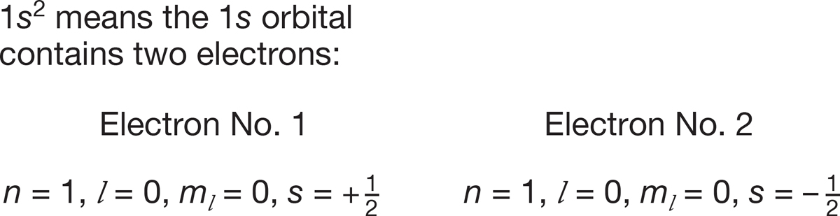
FIGURE 1.4 Two electrons in the same orbital must have opposite (paired) spins.
CONVENTION ALERT
The “1” Is Understood
In Table 1.6, we see the entry 1s 2, which means there are two electrons in the 1s orbital. It would seem that 1s1 would be the appropriate notation for a 1s orbital occupied by one electron. That notation is rarely used, however, and the superscript “1” is almost always understood.
1.2b Electronic Configurations We can now use the quantum numbers n, l, ml, and s to write electronic descriptions, called configurations, for atoms using what is known as the aufbau principle (aufbau is German for “building up” or “construction”). This principle simply makes the reasonable assumption that we should fill the available orbitals in order of their energies, starting with the lowest-energy orbital. To form these descriptions of neutral atoms, we add electrons until they are equal to the number of protons in the nucleus. Table 1.6 gives the electronic configurations of H, He, Li, Be, and B.
TABLE 1.6 Electronic Descriptions of Some Atoms
Atom | Electronic Configuration |
1H |
1s |
2He |
1s2 |
3Li |
1s22s |
4Be |
1s22s2 |
5B |
1s22s22px |
For carbon, the atom after boron in the periodic table, we have a choice to make in adding the last electron. The first five electrons are placed as in boron, but where does the sixth electron go? One possibility would be to put it in the same orbital as the fifth electron to produce the electronic configuration 6C = 1s22s22px2 (Fig. 1.5a). In such an atom, the spins of the two electrons in the 2px orbital must be paired (opposite spins).
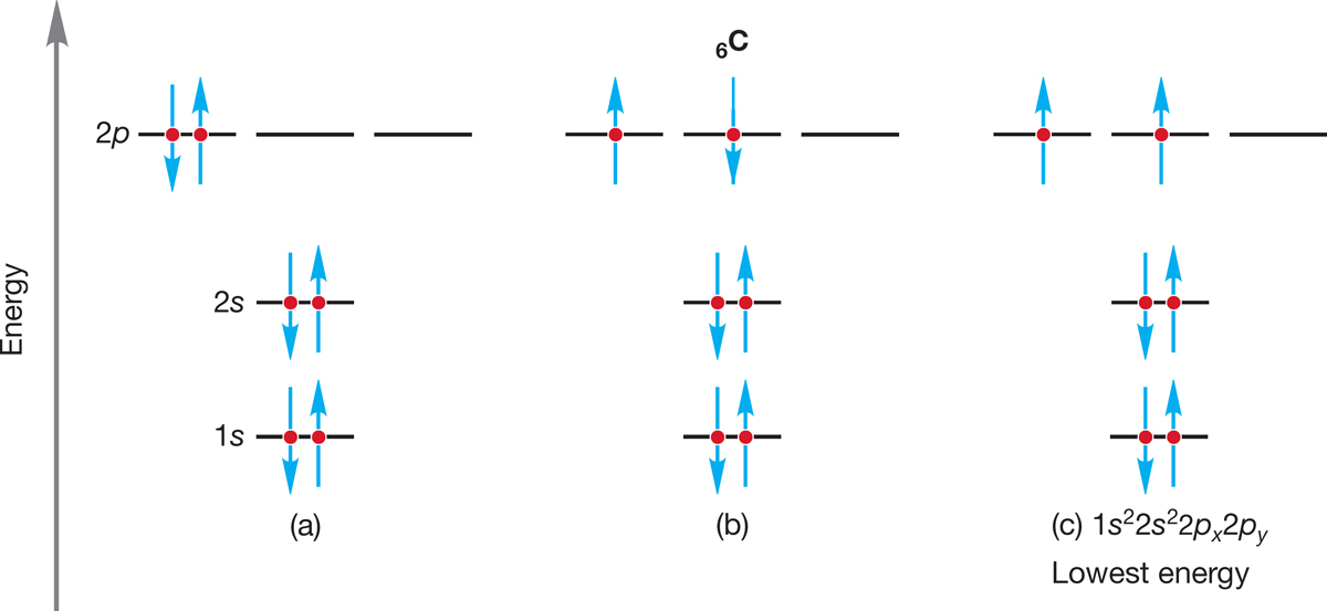
FIGURE 1.5 An application of Hund’s rule. The electronic configuration with the largest number of parallel (same direction) spins is lowest in energy. Note use of the arrow convention to show electron spin.
WORKED PROBLEM 1.1 Explain why the two electrons in the 2px orbital of carbon (6C = 1s22s22px2) must have paired spins (+1/2 and −1/2).
ANSWER6 Because they are in the same orbital (2px), both electrons have the same values for the three quantum numbers n, l, and ml (n = 2, l = 1, ml = +1, 0, or −1). If the spin quantum numbers were not opposite, one +1/2, the other −1/2, the two electrons would not be different from each other! The Pauli principle (no two electrons may have the same values of the four quantum numbers) ensures that two electrons in the same orbital must have different spin quantum numbers.
Alternatively, the sixth electron in the carbon atom could be placed in another 2p orbital to produce 6C = 1s22s22px2py (Fig. 1.5b). The only difference is the presence of two electrons in a single 2p orbital (6C = 1s22s22px2) in Figure 1.5a versus one electron in each of two different 2p orbitals (6C = 1s22s22px2py) in Figure 1.5b. The three 2p orbitals are of equal energy (because each has n = 2, l = 1), so how should we make this choice? Electron–electron repulsion would seem to make the second arrangement the better one, but there is still another consideration. When two electrons occupy different but equi-energetic orbitals, their spins can either be paired (⇅) or unpaired (⇈). Hund’s rule (Friedrich Hund, 1896–1997) holds that for a given electron configuration, the state with the greatest number of unpaired (parallel) spins has the lowest energy. So the third possibility for carbon’s sixth electron (Fig. 1.5c) is actually the best one in this case. Essentially, giving the two electrons the same spin (⇈) ensures that they cannot occupy the same orbital and tends to keep them apart. So, Hund’s rule tells us that the configuration 6C = 1s22s22px2py with parallel spins for the two electrons in the 2p orbitals is the lowest-energy state for a carbon atom.
PROBLEM 1.2 Explain why the fifth and sixth electrons in a carbon atom may not occupy the same orbital as long as they have parallel spins.
Now we can write electronic configurations for the rest of the atoms in the second row of the periodic table (Table 1.7). Notice that for nitrogen we face the same kind of choice just described for carbon. Does the seventh electron go into an already occupied 2p orbital or into the empty 2pz orbital? The configuration in which the 2px, 2py, and 2pz orbitals are all singly occupied by electrons that have the same spin is lower in energy than any configuration in which a 2p orbital is doubly occupied. Again, Hund rules!
TABLE 1.7 Electronic Descriptions of Some Atoms in the Second Row
Atom |
Electronic Configuration |
6C |
1s22s22px2py |
7N |
1s22s22px2py2pz |
8O |
1s22s22px22py2pz |
9F |
1s22s22px22py22pz |
10Ne |
1s22s22px22py22pz2 |
PROBLEM 1.3 Write the electronic configurations for 11Na, 13Al, 15P, 16S, and 18Ar.
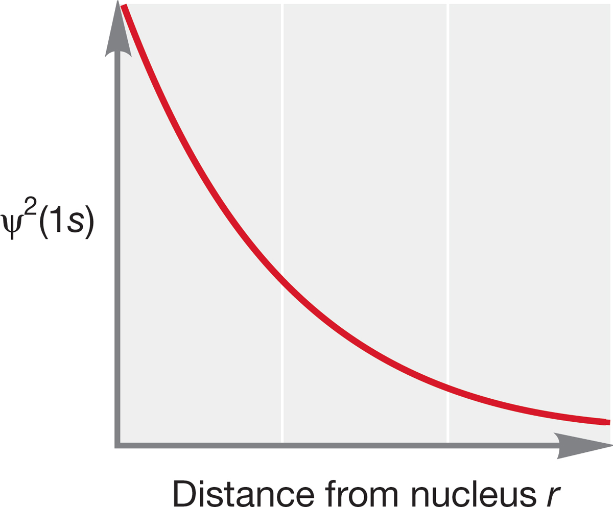
FIGURE 1.6 A plot of ψ2(1s) versus distance r for hydrogen. Note that the value of ψ2 does not go to zero, even at very large r.
To understand the properties and reactions of the molecules you will encounter in organic chemistry, it will be necessary to know the shapes of the molecules. It turns out that molecular shape can be best understood by knowing where the electrons are. Recall that ψ2 is related to the electron density around a nucleus. Therefore, a graph that plots ψ2 as a function of r, the distance from the nucleus, can describe the shape of the orbital. Figure 1.6 plots ψ2 as a function of r for the lowest-energy solution to the Schrödinger equation, which describes the 1s orbital. The graph shows that the probability of finding an electron falls off sharply in all directions (x, y, and z) as we move out from the nucleus. Because there is no directionality to r, we find the 1s orbital is symmetrical in all directions; that is, it is spherical. As noted earlier, the quantum number l is associated with orbital shape, and all s orbitals, for which l always equals zero, are spherically symmetric. Note also that the electron density never goes to zero—a finite (though very, very small) probability exists of finding an electron at a distance of several angstroms (Å; 1.0 Å = 0.10 nm = 1.0 × 10⁻¹⁰ meters) from the nucleus.
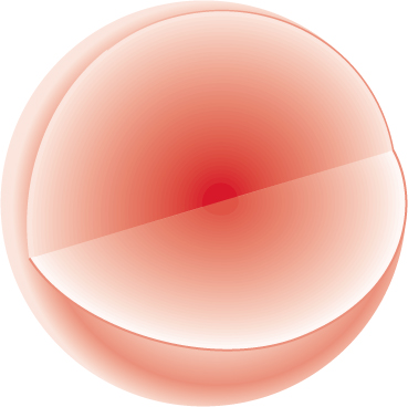
FIGURE 1.7 A three-dimensional picture of the 1s orbital. The surface of the sphere denotes an arbitrary cutoff.
Figure 1.7 translates the two-dimensional graph of Figure 1.6 into a three-dimensional picture of the 1s orbital, a spherical cloud of electron density that has its maximum near the nucleus. Although this cloud of electron density is shown as bound by the spherical surface at some arbitrary distance from the nucleus, it does not really terminate sharply there. This spherical boundary surface simply indicates the volume within which we have a high probability of finding the electron. We can choose to put the boundary at any percentage we like—the 95% confidence level, the 99% confidence level, or any other value. It is this picture that we have been approaching throughout these pages. The representation of the electron density in Figure 1.7 is the one you will probably remember best and the one that will be most useful in our study of chemical reactions. This sphere centered on the nucleus is the region of space occupied by an electron in the 1s orbital.
Figure 1.6 correctly gives the probability of finding an electron at a particular point a distance r from the nucleus, but it doesn’t recognize that as r increases, a given change in r (denoted by the symbol Δr) produces a greater volume of space and thus a greater number of points where the electron might be. To see why this is so, look at Figure 1.8. Even though the increase, Δr, for each concentric circle is the same, the volume is much greater for the outer spherical shell. The change in volume is not linear with the change in radius. Note that the radius for the 1s orbital has its highest probability at 0.53 Å.
We account for this increasing influence of Δr with the graph shown in Figure 1.8. Here, the horizontal axis is again r, but the vertical axis (4πr2ψ2) accounts for the volume of the sphere. The resulting graph gives a picture of the probability of finding an electron at all points at a distance r from the nucleus. This new picture takes account of the increasing volume of spherical shells of thickness Δr as the distance from the nucleus, r, increases.
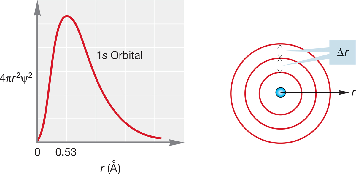
FIGURE 1.8 The graph on the left shows a slice through the three-dimensional 1s orbital. At relatively low values of r (short distance from the nucleus), Δr will contain a smaller volume than at higher values of r (larger distance from the nucleus). The outer spherical shell contains a greater volume than the middle shell even though they are both Δr wide. This plot is weighted for the increasing influence of Δr as r gets larger.
Summary
1. An electron is described by four quantum numbers (n, l, ml, and s).
2. Electrons are filled into the available orbitals starting with the lowest-energy orbital (the aufbau principle).
3. An orbital can contain only two electrons, which must have paired spin quantum numbers, s = +1/2 and s = −1/2.
4. The quantum number l specifies the shape of the orbital, and all s orbitals have spherical symmetry.
5. We can do no better than to say that with some degree of certainty, an electron is within a certain volume of space. The shape of that volume is given by ψ2.
6. The cutoff point for our degree of certainty is arbitrary because, as Figures 1.6 and 1.8 show, the chance of an electron being far from the nucleus is never zero.
1.2c Shapes of Atomic Orbitals As noted earlier, the mathematical function ψ that describes an atomic orbital has many of the properties of waves. For example, hills and valleys are evident in waves in liquids and in a vibrating string. Hills correspond to regions for which the mathematical sign of ψ is positive, and valleys correspond to regions for which the mathematical sign of ψ is negative. In a vibrating string, when we pass from a length of string in which the amplitude is positive to one where it is negative, we find a stationary point called a node. Nodes also appear in wave functions at the points at which the sign of ψ changes, where ψ = 0. Of course, if ψ = 0, then ψ2 = 0, so the probability of finding an electron at a node is also zero. In an atomic orbital, therefore, a node is a region of space in which the electron density is zero. The number of nodes in an orbital is always one fewer than n, the principal quantum number. Thus, the n = 1 orbital (1s) has no nodes, all n = 2 orbitals have a single node, all n = 3 orbitals have two nodes, and so on. As we turn our attention from the 1s orbital to higher-energy orbitals, we will have to pay attention to the presence of nodes.
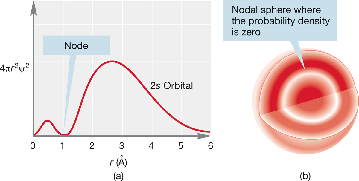
FIGURE 1.9 (a) A plot of 4πr2ψ2 versus r for a 2s orbital and (b) a cross section through the orbital.
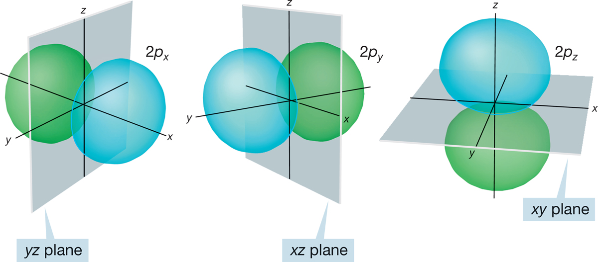
FIGURE 1.10 An accurate three-dimensional representation of three 2p orbitals. Note the nodal planes separating the lobes where the sign of ψ differs. Color is used to emphasize the opposite signs of the lobes.
The next higher energy orbital is the 2s (n = 2, l = 0). Because n = 2, there must be a single node in this orbital, and we expect spherical symmetry, as with all s orbitals. Figure 1.9a shows a plot of 4πr2ψ2 versus r. Figure 1.9b is a three-dimensional representation of the 2s orbital, which shows a spherical node, representing the spherical region at which ψ and ψ2 are zero.
When n = 2, l can equal 1 as well as zero. As described on p. 8, the quantum number combination of n = 2, l = 1 gives the 2px, 2py, and 2pz orbitals, each of which must possess a single node. Because l is not zero, the 2p orbitals are not spherically symmetrical. As you may have guessed from the x, y, z designations, the 2p orbitals are directed along the x, y, and z axes of a Cartesian coordinate system (Fig. 1.10). Each 2p orbital is made up of two lobes that are slightly flattened spheres, and the orbital as a whole is shaped roughly like a dumbbell. The node is the plane separating the two halves of the dumbbell. In one lobe of the orbital, the sign of the wave function is positive; in the other the sign is negative. To avoid confusion with electrical charge, these signs are usually indicated by a change of color rather than + and −. The three 2p orbitals together are shown in Figure 1.11. As you can see, the stylized dumbbells used to represent 2p orbitals are easier to draw than the more accurate picture shown in Figure 1.10.
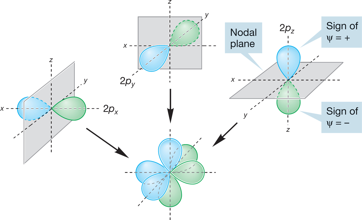
FIGURE 1.11 A schematic three-dimensional representation of three 2p orbitals shown separately and in combination.
For the first time, we begin to get hints of the causes of the complicated three-dimensional structures of molecules: Electrons are the “glue” that holds the atoms of molecules together, and electrons are confined to regions of space that are by no means always spherically symmetrical.
As Figure 1.12 shows, we can now make quite detailed pictures of the electrons in atoms. The 1s orbitals have been omitted in the atoms past He. The other electrons are shown as dots.
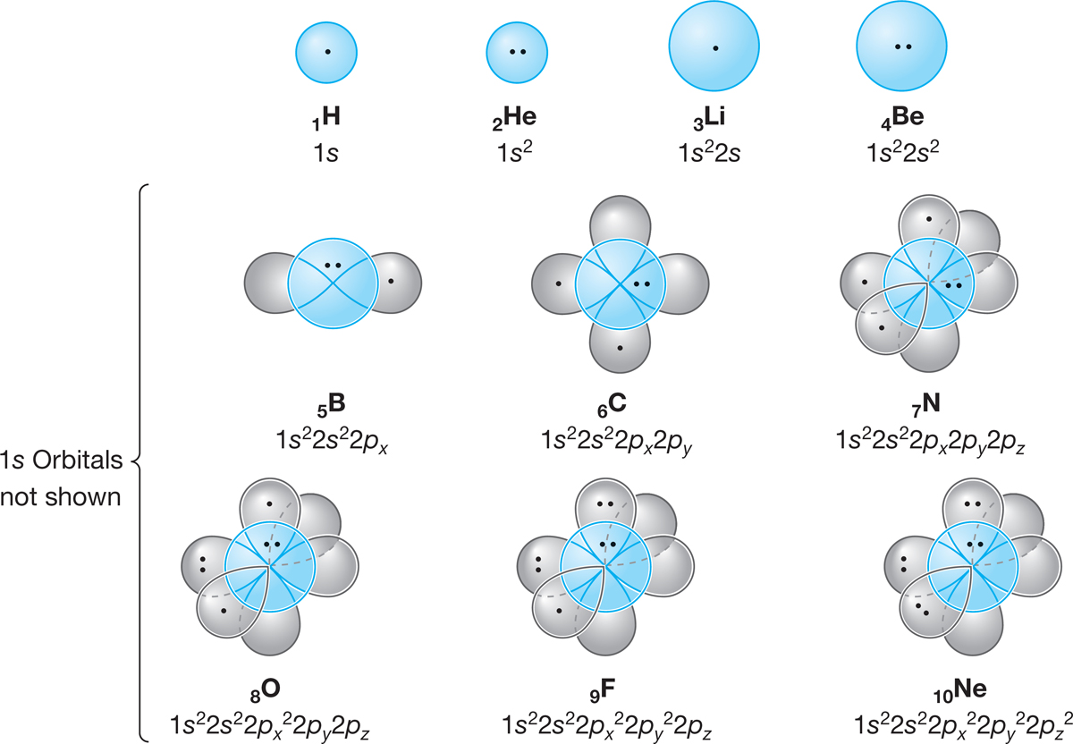
FIGURE 1.12 Schematic illustrations of the first 10 atoms in the periodic table. Each dot represents an electron, although the 1s electrons for the atoms past He are not shown.
Summary
Electrons in atoms are confined to certain volumes of space, and these volumes are not all alike in shape. A dumbbell-shaped 2p orbital is quite different from a spherical 2s orbital, for example.
5There are several units of energy in use. Organic chemists commonly use kilocalories per mole (kcal/mol); physicists use the electron volt (eV). One electron volt/molecule translates into about 23 kcal/mol. Recently, the International Committee on Weights and Measures suggested that the kilojoule (kJ) be substituted for kilocalorie. So far, organic chemists in some countries, including the United States, seem to have resisted this suggestion. We will provide kcal/mol and parenthetical kJ/mol values throughout the text (1 kcal is equal to 4.184 kJ).
6Worked Problems are answered in whole or in part in the text. When only part of a problem is worked, that part will have an asterisk. Complete answers can be found in the Study Guide.